Jane Street Puzzle: Robot Javelin
Problem Statement
It’s coming to the end of the year, which can only mean one thing: time for this year’s Robot Javelin finals! Whoa wait, you’ve never heard of Robot Javelin? Well then! Allow me to explain the rules:
- It’s head-to-head. Each of two robots makes their first throw, whose distance is a real number drawn uniformly from $[0, 1]$.
- Then, without knowledge of their competitor’s result, each robot decides whether to keep their current distance or erase it and go for a second throw, whose distance they must keep (it is also drawn uniformly from $[0, 1]$).
- The robot with the larger final distance wins.
This year’s finals pits your robot, Java-lin ($J$), against the challenger, Spears Robot ($S$). Now, robots have been competing honorably for years and have settled into the Nash equilibrium for this game. However, you have just learned that Spears Robot has found and exploited a leak in the protocol of the game. They can receive a single bit of information telling them whether their opponent’s first throw (distance) was above or below some threshold $d$ of their choosing before deciding whether to go for a second throw. Spears has presumably chosen d to maximize their chance of winning — no wonder they made it to the finals!
Spears Robot isn’t aware that you’ve learned this fact; they assume Java-lin is using the Nash equilibrium strategy.. If you were to adjust Java-lin’s strategy to maximize its odds of winning given this, what would be Java-lin’s updated probability of winning?
Solution
This problem naturally has three components:
- What is the Nash equilibrium strategy in the vanilla game?
- Given that $S$ can see if $J$’s throw was more or less than $d$, what is their optimal $d^*$?
- Knowing that $S$ will play optimally with their new information but doesn’t know $J$ is aware of $S$’s strategy, what is the optimal strategy for $J$ now?
Part 1: Vanilla Nash Equilibrium
We assume both robots use a threshold strategy and by symmetry they adopt the same threshold $\tau$. That is, both robots throw their first javelin. If they throw it further than distance $\tau$ then they keep their first throw, otherwise they throw again. In this first part, we’ll find the value of $\tau$.
Recall that in a Nash equilibrium, no player can unilaterally change their strategy and improve their position. So without loss of generality, let’s assume that $J$ uses $\tau$ and $S$ uses $t$. We would like to find the value of $\tau$ such that for all $t \in [0, 1]$, $S$’s probability of winning is maximized at $t = \tau$.
To do this, we first need an expression for the probability that $S$ wins given they use strategy $t$ and $J$ uses strategy $\tau$. Let $\tilde{s}$ and $\tilde{j}$ be random variables denoting the distance $S$ and $J$ use in their score respectively. We want to determine $\Pr[\tilde{s} > \tilde{j}]$. We can write down the CDF of $\tilde{s}$ for fixed $t$ as :
\(\begin{equation*} F_S(s, t) = \begin{cases} t s & 0\leq s\leq t \\ (s-t) + s t & t<s<1. \end{cases} \end{equation*}\) This follows from the fact that the only way to throw at most $s$ for $s \leq t$ is to throw under $t$ the first throw, then under $s$ the second. And for $s > t$ we can throw between it and $t$ on our first throw with probability $s - t$ or below $t$ on the first throw and then under $s$ the second. By the same logic, the CDF of $\tilde{j}$ is
\[\begin{equation*} F_J(j) = \begin{cases} \tau j & 0\leq j\leq \tau \\ (j-\tau) + j \tau & \tau<j<1. \end{cases} \end{equation*}\]With these, we can write $\Pr[\tilde{s} > \tilde{j}]$ as a function of $t$.
\[\begin{equation} \begin{aligned} \Pr\left[\tilde{s} > \tilde{j}\right](t, \tau) & = \int_{0}^1 F_J(s) f_s(s, t) \; ds \\ & = \begin{cases} \frac{1}{2} \left(\tau ^2-\tau -\tau t^2+\left(\tau ^2-\tau +1\right) t+1\right) & 0\leq t \leq \tau \\ \frac{1}{2} \left(-\tau -\left((\tau +1) t^2\right)+\left(\tau ^2+\tau +1\right) t+1\right) & \tau<t<1. \end{cases} \end{aligned}\label{eq:van_nash} \end{equation}\]Now, we would like to find the value of $\tau$ such that: $\Pr \left[\tilde{s} > \tilde{j}\right](t, \tau)$ is maximized in $t$ at $t = \tau$. If we vary $\tau$ and plot the probability of winning as a function of $t$, we can see that there is some $\tau$ for which the function in $t$ is strictly decreasing in $t$ on either side of $t = \tau$.
Taking the derivative of (\ref{eq:van_nash}) in $t$, setting $t = \tau$, and then solving for the root in $\tau$ yields a value of
\[\begin{equation*} \boxed{\tau = \frac{\sqrt{5} - 1}{2}} \end{equation*}\]which is the unique Nash-equilibrium threshold strategy in the vanilla game and aligns with the value we would expect from Figure 1.
Part 2: Optimal Cheating
The next step is to determine what value of $d$ player $S$ should use to cheat in an optimal way. Recall that $S$ is choosing $d$ with the belief that $J$ is using the vanilla strategy with threshold $\tau$.
To choose $d$, $S$ can utilize two pieces of information: their initial throw value and a bit indicating whether or not $J$’s first throw exceeded $d$. From this information, $S$ must decide to rethrow or keep. Like in the previous section, we will develop an expression for the probability $S$ wins when $d \leq \tau$ and $d > \tau$ and use those to determine an optimal value for $d$.
Case 1: $d < \tau$
Suppose $d \leq \tau$ and $S$’s initial throw was $s_1$. We can break up the probability $S$ wins by considering the cases where $J$’s first throw, denoted $j_1$, was more or less than $d$. If $j_1 < d \leq \tau$, then $S$ knows that $J$ will rethrow. In that case, $S$ will keep if their initial throw was at least $1/2$ and rethrow otherwise. Therefore, the probability of $S$ winning if they initially throw $s$ and observe that $j_1 < d$ is $P_{lo}(s_1) = \max(s_1, 1/2)$ where the first term represents keeping their initial throw of $s$ and the second is the event they both rethrow.
On the other hand, if $j_1 > d$ then since $d \leq \tau$, $J$ may rethrow or keep. If $S$ keeps here, they win with probability
By the same conditioning logic, we find that if $S$ rethrows they win with probability
$S$ will choose the larger of $P_{keep}(s_1)$ and $P_{throw}$ depending on the value of $s_1$.
Putting it together and integrating these cases over the possible values of $s_1$, the probability of $S$ winning for a given $d \leq \tau$ is
\[\begin{equation*} \begin{aligned} P_{Win (d < \tau)}(d) & = \int_{0}^1\bigg( d \cdot P_{lo}(s_1) + (1 - d)\cdot \max\bigg\{P_{keep}(s_1), P_{throw} \bigg\}\bigg) \; d s_1 \\ & = \frac{\left(19-5 \sqrt{5}\right) d^2-\left(11 \sqrt{5}+1\right) d+4 \left(\sqrt{5}+3\right)}{4 \left(-2 d+\sqrt{5}+1\right)^2} \end{aligned} \end{equation*}\]Case 2: $d > \tau$
Now, we must perform the same analysis for $d > \tau$. If $S$ observes that $j_1 \geq d \geq \tau$, then they will know $J$ will keep with certainty. If $S$ rethrows they win with probability $(1 - d)/2$, and if they keep, they win with probability $\max ( 0, (s_1 - d)/(1 - d) )$. Putting these together, in the event that $S$ observes that $J$ throws more than $d$, $S$ wins with probability
Next, in the event $S$ observes $j_1 < d$, $J$ may rethrow or keep, so we need to use the same conditioning logic as in the previous case. Doing so, we find that the probability of $S$ winning when they keep and rethrow are:
As for a brief explanation of the terms in $P_{keep}(s_1)$, note since $j_1 < d$, $J$ will rethrow with probability $d/\tau$ and then the second throw will be less than $s_1$ with probability $s_1$. That is why the term $\tau s_1/d $ appears in each case. The last two terms consider the additional case where $J$ keeps. For the middle term, some $j_1$ can beat $s_1$ in this interval; whereas in the last term, since $s_1 > d > j_1$, $S$ wins.
Similar to in the previous case, $S$ will choose the larger of the two options $P_{keep}(s_1)$ and $P_{throw}$. We can now integrate the probability of winning when $d > \tau$ as a function of $s$ to get \(\begin{equation*} \begin{aligned} P_{Win (d > \tau)}(d) & = \int_{0}^1\bigg( d \cdot P_{hi}(s_1) + (1 - d) \cdot \max\bigg\{P_{keep}(s_1), P_{throw} \bigg\} \bigg)\;ds_1 \\ & = \frac{\left(\sqrt{5}+1\right) d^4-8 d^3+2 \left(\sqrt{5}+1\right) d^2-8 \left(\sqrt{5}-2\right) d+9 \sqrt{5}-15}{8 \left(\sqrt{5}-1\right)} \end{aligned} \end{equation*}\)
If we now plot the probability of $S$ winning as a piecewise function in $d$ consisting of $P_{Win (d < \tau)}(d)$ and $P_{Win (d > \tau)}(d)$, we see:
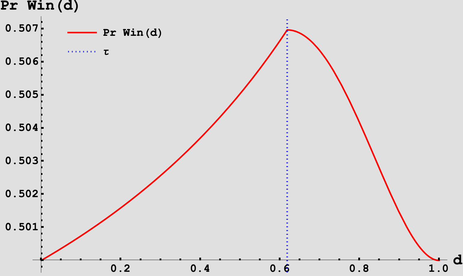
this implies that $\boxed{d^* = \tau}$. We can then further verify this by noting that the derivatives of $P_{Win (d < \tau)}(d)$ and $P_{Win (d > \tau)}(d)$ are strictly increasing and decreasing in $d$ for their respective regions.
The takeaway is that the optimal query is simply whether $J$ will rethrow. When $S$ does this, they win with probability
\[\Pr[S \text{ win}](d^*) = \frac{1}{8} \left(13-4 \sqrt{5}\right) \approx 0.506966.\]Which is a slight edge above the previous 50-50 outcome.
Part 3: $J$’s Optimal Response to Cheating
Lastly, $J$ knows that $S$ can tell if $J$’s first throw is below or above $\tau$. How can $J$ use this information to devise an optimal response to $S$’s cheating? $S$’s behavior will vary depending on whether or not $J$’s first throw was more or less than $\tau$. We can assume $J$ uses a threshold strategy that depends on the first throw. Let $r$ be the new threshold used by $J$.
First suppose that $j_1 \leq \tau$ . When should $J$ keep the first throw?
Since $S$ is cheating, they know $j_1 \leq \tau$. Based on the strategy we discovered in the previous part the CDF of the final value $S$ receives is
\[\begin{equation*} F_S(s) = \begin{cases} \frac{s}{2} & 0\leq s \leq \frac{1}{2} \\ \frac{3 s}{2}-\frac{1}{2} & \frac{1}{2}\leq s \leq 1 . \end{cases} \end{equation*}\]For fixed threshold $r < \tau$ we can develop the corresponding CDF and PDF for $J$’s final value
\[\begin{equation*} F_J(j, r) = \begin{cases} \frac{r j}{\tau } & 0\leq j\leq r \\ \frac{r j}{\tau } + \frac{j-r}{\tau } & r\leq j\leq \tau \\ \frac{r j}{\tau } + 1 - \frac{r}{\tau} & \tau \leq j\leq 1 \\ \end{cases} \end{equation*}\] \[\begin{equation*} f_J(j, r) = \begin{cases} \frac{r}{\tau } & 0\leq j\leq r \\ \frac{r + 1}{\tau } & r\leq j\leq \tau \\ \frac{r}{\tau } & \tau \leq j\leq 1 \\ \end{cases}. \end{equation*}\]Thus, the probability of $J$ winning as a function of $r$ is
\[\begin{equation*} \Pr\left[ J \text{ win}| j_1 \leq \tau\right](r) = \int_0^1 F_S(j) \cdot f_J(j) \;dj. \end{equation*}\]We visualize this below in Figure 3.
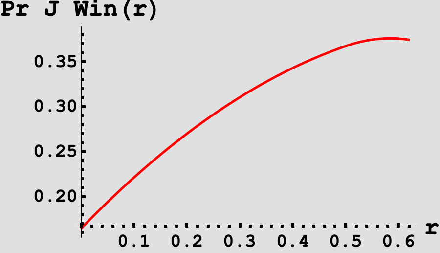
From the figure, we see that the function seems to be unimodal with a maximum somewhere just before the threshold. Sure enough, if we take the derivative and solve for the root, we find that $\boxed{r^* = 7/12}$ is the optimal threshold strategy for $J$ when $j_1 \leq \tau$ which yields
\[\begin{equation*} \Pr\left[J \text{ win}| j_1 \leq \tau\right](r^*) =\frac{\frac{313}{24}-5 \sqrt{5}}{4 \left(\sqrt{5} - 1\right)}. \end{equation*}\]In summary, there is now a window, $[7/12, \tau]$, such that when $J$’s first throw falls in this window, $J$ can take advantage of $S$’s cheating and keep when $S$ thinks that $J$ will rethrow.
In the event that $j_1 > \tau$, we can suppose another threshold $r’$ and repeat the same steps as before. However, this time we find that $\Pr\left[J \text{ win}\mid j_1 > \tau\right](r’)$ is a strictly decreasing function for $r’ \geq \tau$, implying that when $J$’s first throw exceeds $\tau$, they should always keep, as in the vanilla strategy. Furthermore, when plugging in $r’ = \tau$, we find that
We have now worked out everyone’s optimal strategy and now it remains to compute the probability that $J$ wins! By conditioning on the event that $J$’s first throw is below or above $\tau$, we finally find
\[\begin{equation*} \begin{aligned} \Pr\left[J \text{ win}\right] & = \Pr\left[J \text{ win}| j_1 \leq \tau\right](r^*) \cdot \Pr[j_1 \leq \tau] + \Pr\left[J \text{ win}| j_1 > \tau\right](\tau) \cdot \Pr[j_1 > \tau] \\ & = \frac{\frac{313}{24}-5 \sqrt{5}}{4 \left(\sqrt{5} - 1\right)} \cdot \tau + \frac{1}{8} \left(2 \sqrt{5}+1\right) \cdot (1 - \tau) \\ & = \boxed{\frac{1}{192} \left(229-60 \sqrt{5}\right)}\\ \end{aligned} \end{equation*}\]How does this fare against the previous odds when $J$ did not know $S$ was cheating? Previously, against cheating $S$, $J$ won with probability $0.493034$ whereas now they win with probability $0.493937$. A very minor improvement. Unfortunately for $J$, $S$’s cheating is hard to recover from. Fortunately for them, the game is still nearly 50-50!
Enjoy Reading This Article?
Here are some more articles you might like to read next: