Can You Throw the Hammer?

This week’s The Fiddler on the Proof puzzle is paraphrased as follows:

You (Player 1) and your opponent (Player 2) are competing in a TGL golf match. On any given hole you play, each of you has a 50-percent chance of winning the hole (and a zero percent chance of tying). That said, scorekeeping in this match is a little different from the norm.

Each hole is worth 1 point. Before starting each hole, either you or your opponent can “throw the hammer.” When the hammer has been thrown, whoever did not throw the hammer must either accept the hammer or reject it. If they accept the hammer, the hole is worth 2 points. If they reject the hammer, they concede the hole and its 1 point to their opponent. Both players can throw the hammer on as many holes as they wish. (Should both players decide to throw the hammer at the exact same time—something that can’t be planned in advance—the hole is worth 2 points.)

The first player to reach \(n\) points wins the match. Suppose all players always make rational decisions to maximize their own chances of winning. If the first player wins the first hole and the score is \((1 - 0)\) what is the probability that they win the match?

Solution

This is a quick one this week! For each round, the players are playing in a zero-sum game.We can view them as competing for the “resource” that is the probability that they win the overall game given the current round. To solve for the probability that Player 1 wins from the score-state \((1,0)\), which we denote as \(V(1, 0)\), we need to develop a recursive relationship for \(V(i, j)\), the probability that the first player wins from state \((i, j)\) (Player 1 has \(i\) points and Player 2 has \(j\) points).

We observe that, at the start of each turn each player has two actions to start the turn: throw the hammer or do not throw the hammer. In the case that they do not throw the hammer, then they may have to then make the secondary choice of “accept” or “reject” if the other player chooses to throw their hammer. We adopt the convention that Player 1 chooses their actions based on the objective of maximizing the probability that they win the overall game at state \((i, j)\), \(V(i, j)\). Conversely, Player 2 chooses actions with the objective of minimizing this \(V(i, j)\). This leads us to the recurrence relation:

With the base case(s) of

Here we can see Player 1 is taking the action that maximizes their probability of winning the game given that, if they took a particular action, Player 2 would choose the action to minimize Player 1’s probability of winning under that action. We see in (\ref{eq:rec}) that in the case Player 1 chooses not to hammer, they may then face a secondary decision to accept or reject a Player 2 hammer toss, in which they would again choose the probability-maximizing action.

We can code this recurrence up in python using Dynamic Programming and visualize the probability of Player 1 winning at any given state. Here we have actually taken the liberty of slightly generalizing the problem. We are assuming that the Player 1’s probability of winning on round \(i + j\) (the current round, zero indexed) is known and is given by a list hole_probs. In the context of our original problem, every entry of hole_probs would be \(1/2\)

from functools import cache

@cache
def V(i, j):
    """ Probability Player 1 wins the game given we are at state (i, j) and they
    are playing to score n. We assume there is some list of probabilities 
    hole_probs such that hole_probs[i + j] is the probability that Player 1
    wins the current hole.  """
    if i >= n:
        return 1
    elif j >= n:
        return 0

    # the prob Player 1 wins current hole   
    p = hole_probs[i + j] 

    # Player 1 hammers
    prob_toss_win = min(
        p * V(i + 2, j) + (1 - p) * V(i, j + 2), 
        V(i + 1, j)
        )

    # Player 1 does not hammer
    prob_pass_win = min(
        p * V(i + 1, j) + (1 - p) * V(i, j + 1),
        max(
            p * V(i + 2, j) + (1 - p) * V(i, j + 2),
            V(i, j + 1)
            )
     )

    return max(prob_toss_win, prob_pass_win)  

# now input problem specific parameters and solve 
n = 5
hole_probs = [1/2 for _ in range(2 * n)]
print(f' The probability of Player 1 winning is {V(1,0)}')

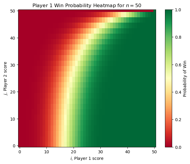
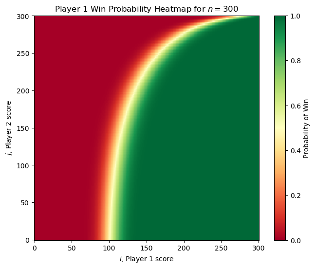
With this, we can get visualize the probability of Player 1 winning from any state. Here are two examples of the original problem (each player is equally skilled) for small and large \(n\).

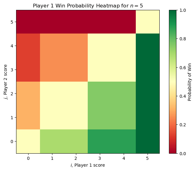
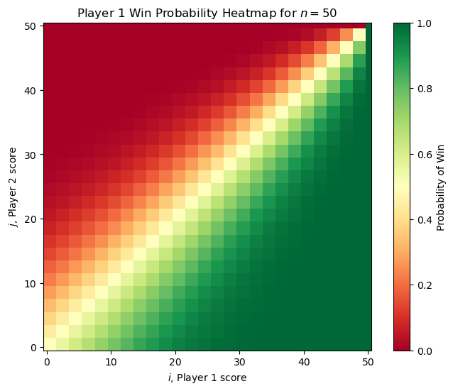
It’s worth noting that the “no hammer” option is never used by either player in this setting. For any \(n\) we can compute the value of \(V(1,0)\) in \(\mathcal{O}(n^2)\) time using our dynamic programming approach. For small \(n\), Player 1 has a significant advantage (for example \(n =3\) has \(V(1, 0) = 3/4\)) but as \(n\) increases, the value of \(V(1, 0)\) approaches \(1/2\) as we might expect.

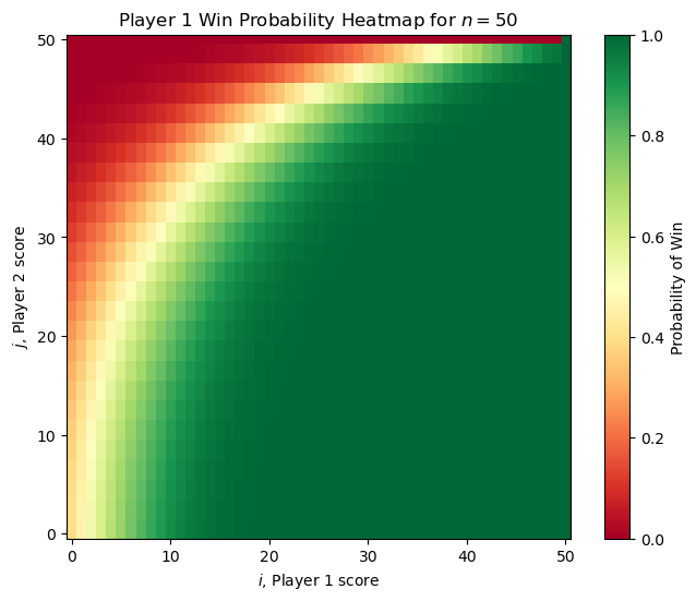
Just for fun, we can also test out a different hole_probs distribution and see how this changes things. One interesting scenario is when Player 1 gradually improves over time. Specifically, at state \((i, j)\) the probability that they win the round is given by

(as the round number increases Player 1 gets linearly better). Initially Player 1 would be very bad and unlikely to win, but in the higher rounds they would be increasingly more clutch over Player 2.

The win‑probability heatmaps now look like the figures below, revealing three asymmetric regions of the state space (one favoring each player and one where they are neutral). In this case, we see the “no hammer” option become used more widely.

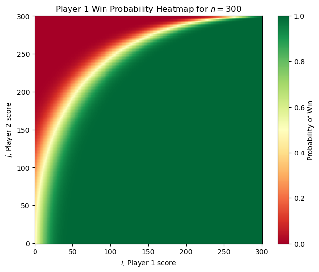
Lastly, here is one more scenario where

Here Player 1 still improves over the rounds but their skill grows quadratically. See if you can come up with your own funky distribution and see what the heatmap looks like using the code above and below!

import matplotlib.pyplot as plt
import numpy as np
n = 5
hole_probs = [1/2 for _ in range(2 * n + 1)]
#hole_probs = [i / (2 * n  - 2) for i in range(2 * n - 1)]
#hole_probs = [np.sqrt(i / (2 * n  - 2)) for i in range(2 * n - 1)]
#hole_probs = [(i / (2 * n  - 2)) ** 2 for i in range(2 * n - 1)]
print(f'for n = {n}, the probability of Player 1 winning from the start is {V(0, 0):.4f} and with a 1 point lead is {V(1, 0):.4f}')
def plot_prob_win_heatmap(n):
    """ heatmap of win probabilities V(i, j) for 0 <= i, j < n."""
    # matrix of V(i, j) 
    M = np.zeros((n + 1, n + 1))
    for i in range(n + 1):
        for j in range(n + 1):
            M[i, j] = float(V(j, i))
    
    # plot the heatmap
    plt.figure(figsize=(8, 6))
    plt.imshow(M, origin='lower', cmap='RdYlGn', interpolation='nearest')
    plt.colorbar(label='Probability of Win')
    plt.xlabel(r'$i$, Player 1 score')
    plt.ylabel(r'$j$, Player 2 score')
    plt.title(fr'Player $1$ Win Probability Heatmap for $n = {n}$')
    plt.show()

# try it out 
plot_prob_win_heatmap(n)