Jane Street Puzzle: Robot Road Trip
Problem Statement
Robot cars have a top speed (which they prefer to maintain at all times while driving) that’s a real number randomly drawn uniformly between $1$ and \(2\) miles per minute. A two-lane highway for robot cars has a fast-lane (with minimum speed \(a\)) and a slow-lane (with maximum speed \(a\)). When a faster car overtakes a slower car in the same lane, the slower car is required to decelerate to either change lanes (if both cars start in the fast-lane) or stop on the shoulder (if both cars start in the slow-lane). Robot cars decelerate and accelerate at a constant rate of $1$ mile per minute per minute, timed so the faster, overtaking car doesn’t have to change speed at all, and passing happens instantaneously.
If cars rarely meet (so you never have to consider a car meeting more than one other car on its trip, see Mathematical clarification below), and you want to minimize the miles not driven due to passing, what should \(a\) be set to, in miles per minute? Give your answer to 10 decimal places.
\[a^* = \lim_{N \to \infty} \lim_{z \to 0^+} f(z,N)\]Mathematical clarification: Say car trips arrive at a rate of $z > 0$ car trip beginnings per mile per minute, uniformly across the infinite highway (cars enter and exit their trips at their preferred speed due to on/off ramps), and car trips have a constant length of \(N\) miles. Define \(f(z,N)\) to be the value of $a$ that minimizes the expected lost distance per car trip due to passing. Find:
Solution
At a high-level, our solution will do the following:
- For car $C$ entering the roadway at a given location, time, and speed, determine the necessary conditions for another car to overtake $C$ during $C$’s journey.
- Determine, for each overtake, the total miles not driven due to passing
- Combine these two to determine the expected miles not driven due to passing for a car traveling at speed $v$.
- Average over all $v$ and determine the optimal speed threshold $f(z, N)$ for the highway.
- Determine $a^* = \lim_{N \to \infty} \lim_{z \to 0^+} f(z,N)$
Before diving into the analysis, we will point out an observation from the mathematical clarification. Suppose we have an infinitely long highway at which cars enter at rate $z$ starts/mile/minute. Based on this description, we can say that the number of cars that enter the highway on a strip of length $\Delta x$ during a duration of time $\Delta t$ is a Poisson random variable with mean/rate $\lambda = z \Delta x \Delta t$. An important property of Poisson random variables is that their sum is also a Poisson random variable in which their rates have been added. With this in mind, we begin our analysis.
Let us consider a car $C$ that enters the highway (WLOG) at $x = 0$ and $t = 0$ with speed $v \in [1, 2]$. This car will travel for $N / v$ minutes and exit the highway at its destination $x = N$. We would like to determine the distribution for the number of cars will catch up to and pass $C$. First some observations. For a car $C’$ to pass car $C$, it must meeting the following conditions:
- Have speed $u > v$ (It is moving faster than $C$).
- If it starts its trip at time $t = t_s$, $C’$ must be behind where $C$ is at $t = t_s$ (It must start behind $C$ to overtake it).
- Share the same position as $C$ at some time $t$ during the time interval at which both cars are driving.
Using these, we would like to get a distribution for the number of cars that will pass $C$. Let us start by fixing the speed of car $C’$, to be some $u$ such that $u > v$. What are the conditions on the starting time and position of $C’$ that will allow it to pass $C$? Suppose $C’$ starts at position $x_s$ at time $t_s$ and the two cars intersect at time $t$. Based the previous conditions, we get the following inequalities:
\[\begin{align} & t_s \leq t \leq t_s + N/u && (\text{intersect while $C'$ exists}) \\ & 0 \leq t \leq N/v && (\text{intersect while $C$ exists}) \\ & x_s + u(t - t_s) = v t && (\text{Both at same location at time $t$}) \label{eq:same_x}. \end{align}\]Using (\ref{eq:same_x}), we can solve for $t$ as $t = \frac{u t_s - x_s}{u - v}$ and plug this into the other inequalities to get a set of four inequalities in the $(x_s, t_s)$-space.
\[\begin{align} & t_s \leq \frac{u t_s - x_s}{u - v} \leq t_s + N/u \\ & 0 \leq \frac{u t_s - x_s}{u - v} \leq N/v \\ \end{align}\]Which when plotted in the $(x_s, t_s)$-space, these inequalities define a region $R$ which is a convex quadrilateral. This region is the set of all pairs of $(x_s, t_s)$ that would allow $C’$, traveling at speed $u$ to intersect $C$. See an example below.
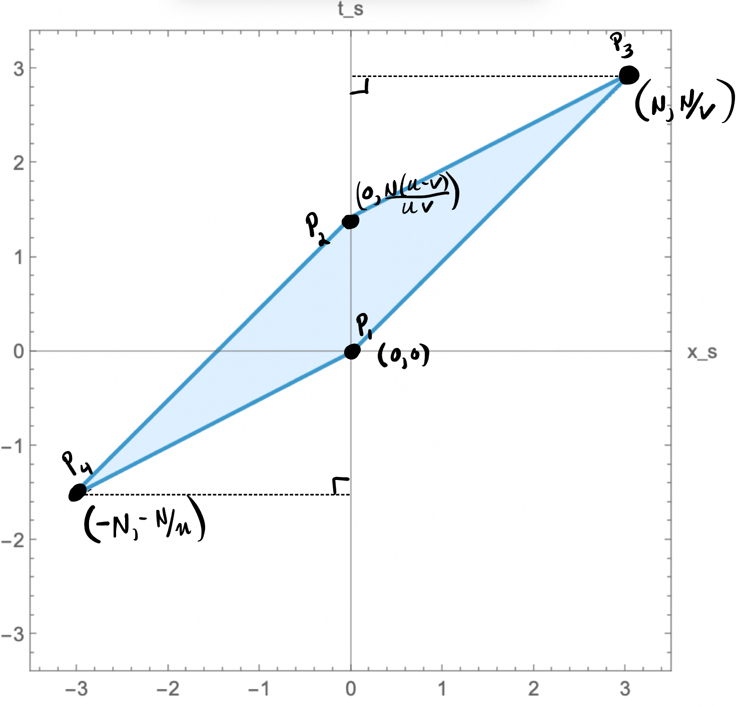
The vertices of $R$ are given by
\[\begin{align*} P_1 & = (0, 0)\\ P_2 & = (0, \frac{N(u - v)}{uv})\\ P_3 & = (N, N/v) \\ P_4 & = (-N, -N/u), \end{align*}\]which imply that the area of our quadrilateral is \(\boxed{ Area(R) = \frac{N^2 (u - v)}{uv}}\).
Using our earlier observation about the number of cars for a given region of time and space being a Poisson random variable with parameter proportional to the area of that region, we deduce that the distribution for the number of which cars of speed $u$ that arrive in the time-space region $R$ is a Poisson random variable with rate parameter $\lambda(u)$ given by
\[\lambda(u) = z dF(u) \frac{N^2 (u - v)}{uv} = z \frac{N^2 (u - v)}{uv} du.\]Where $z dF(u)$ is the rate at which car of speed $u$ arrive per mile per minute. Since the speed of cars is distributed $U(1, 2)$, we have $dF(u) = du / 1$.
We now have enough to compute the rate of overtakes for $C$ when it is in the slow-lane $\Lambda_S$ and when it is in the fast-lane, $\Lambda_F$.
For the slow-lane, we have
\[\begin{align*} \Lambda_S & = \int_v^a z \frac{N^2 (u - v)}{uv} du \\ & = \frac{N^2 z \left(a - v \log \left(\frac{a e}{v}\right)\right)}{v}. \end{align*}\]And for the fast-lane
\[\begin{align*} \Lambda_F & = \int_v^2 \frac{N^2 (u - v)}{uv} du \\ & = \frac{N^2 z \left(2 -v \log \left(\frac{2e}{v}\right)\right)}{v}. \end{align*}\]These are the expected number of intersections per trip for a car of speed $v$, depending on whether the car is in the slow-lane or the fast-lane (since they are Poisson random variables). Now, we need to determine the “loss of distance traveled” for each overtake in either scenario.
Suppose we are in the slow-lane. Whenever we are passed, we must fully stop and then speed up to speed $v$ again. Since the acceleration is fixed to be $1$, the time it take to stop and speed up are the same and is $\delta t = v$ minutes. The total distance that would be traveled during this time without intersection is
\[d_0 = v(\delta t + \delta t) = 2 v^2.\]On the other hand, when we have to stop, the distance traveled during the deceleration is
\[d_1 = v \delta t - \frac{1}{2}(\delta t)^2 = v^2 / 2,\]and acceleration
\[d_2 =\frac{1}{2}(\delta t)^2 = v^2 / 2.\]Thus the “loss of distance” for each passing in the slow-lane is:
\(\boxed{d_0 - d_1 - d_2 = v^2}\).
By similar calculations, we find the “loss of distance” per passing in the fast-lane is:
\[\boxed{(v - a)^2}.\]Putting these together, for a car of speed $v$ the expected lost distance due to passing, $\ell(v)$, is given by:
\[\begin{align*} \boxed{ \ell(v) = \begin{cases} v^2 \cdot \frac{N^2 z \left(a - v \log \left(\frac{a e}{v}\right)\right)}{v} & v \leq a \\ (v - a)^2 \cdot \frac{N^2 z \left(2 -v \log \left(\frac{2e}{v}\right)\right)}{v} & v > a \end{cases}} \end{align*}\]Since the speed of cars is distributed $U(1, 2)$, we need to compute the expected total lost distance for a car entering the highway with speed threshold $a$, denoted $L(a)$. We find
\[\begin{align*} L(a) & = \int_{1}^2 \ell(v)\; d v \\ & =\frac{1}{18} N^2 z \bigg(a^3 (18+\log (64))+18 a^2 (\log (4)-1)-6 \left(a^3+6 a^2-1\right) \log (a)-45 a+16\bigg). \end{align*}\]Now, for fixed $z$ and $N$, we would like to find the value of $a$ that minimizes the above expression. However, note that $N$ and $z$ simply contribute a positive scaling factor and do not affect minimizing the overall expression. Therefore, it suffices to remove the constant factors and instead minimize the function
\[g(a) := a^3 (18+\log (64))+18 a^2 (\log (4)-1)-6 \left(a^3+6 a^2-1\right) \log (a)-45 a+16.\]If we plot $g(a)$ over the interval $a \in [1,2]$, (see Figure 2) it appears that the function should have a unique minimizer over the desired interval.

Unfortunately, there is not a nice closed form solution for the minimizer, so we will have to solve for it numerically. Doing so yields for fixed $N$ and $z$,
\[\begin{equation*} \boxed{f(z, N) = 1.177141417} \end{equation*}\]taking the limit of which for $N$ and $z$ has no effect, and thus we have found the value of $a^*$ that minimizes the expected lost distance due to passing.
This value is pretty close to the minimum end of possible speeds on the highway! Around $82\%$ of the cars, on the highway are in the fast-lane. Why might that be? Well we can note that it is pretty expensive for a car in the slow-lane to be passed. Since $v \geq 1$ the loss of distance for every car in the slow-lane is at least $1$ whereas the maximum penalty for a passing in the fast-lane is at most 1. We see that passings in the slow-lane are much more expensive and thus we would need to have fewer of them than in the fast-lane in an optimal solution.
This was a fun problem that had me brushing up on my Poisson processes. I even found several problems in the Poisson Process section of Sheldon Ross’s Stochastic Processes textbook that were about cars entering a highway according to a similar rule which served as a great warm-up to tackling this problem!
Enjoy Reading This Article?
Here are some more articles you might like to read next: