<?xml version="1.0" encoding="utf-8"?><feed xmlns="http://www.w3.org/2005/Atom" xml:lang="en"><generator uri="https://jekyllrb.com/" version="4.4.1">Jekyll</generator><link href="https://ccolombe12.github.io/feed.xml" rel="self" type="application/atom+xml" /><link href="https://ccolombe12.github.io/" rel="alternate" type="text/html" hreflang="en" /><updated>2026-10-08T05:35:47+00:00</updated><id>https://ccolombe12.github.io/feed.xml</id><title type="html">blank</title><subtitle>The academic webpage of Connor Colombe
</subtitle><entry><title type="html">Jane Street Puzzle: Andy’s Afternoon Amble</title><link href="https://ccolombe12.github.io/blog/2026/JS_Andys_Amble/" rel="alternate" type="text/html" title="Jane Street Puzzle: Andy’s Afternoon Amble" /><published>2026-09-01T12:00:00+00:00</published><updated>2026-09-01T12:00:00+00:00</updated><id>https://ccolombe12.github.io/blog/2026/JS_Andys_Amble</id><content type="html" xml:base="https://ccolombe12.github.io/blog/2026/JS_Andys_Amble/"><![CDATA[<h1 id="problem-statement">Problem Statement</h1>

<figure>

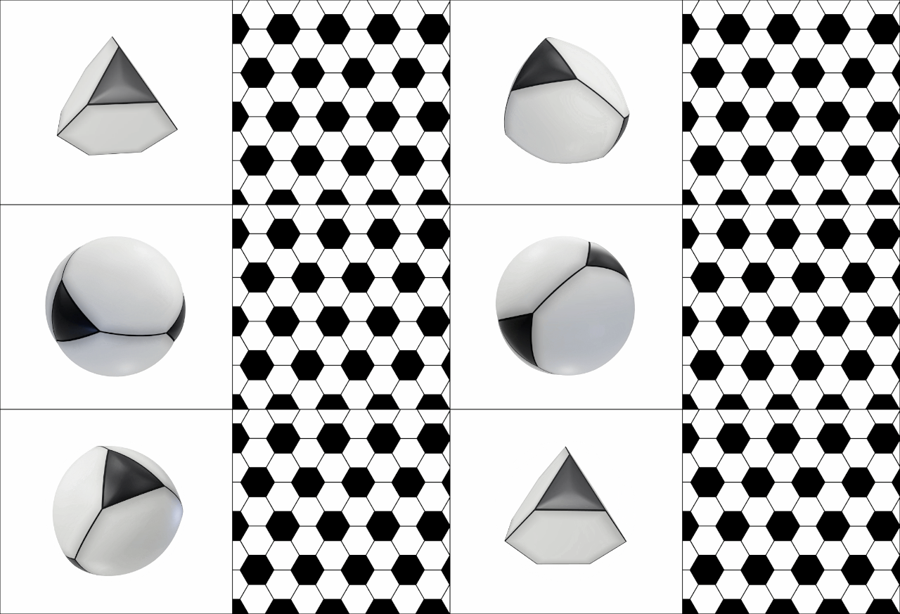
  <img src="/assets/img/blog_images/2026-10-07-andys-amble/andys-afternoon-amble.gif" alt="Truncated tetrahedral sphere and hexagonal floor tiling" width="80%" style="display: block; margin: auto;" />
     <figcaption style="text-align: center; font-style: italic; font-size: 0.9em; color: #666;"> The puzzle's figure: Andy's truncated tetrahedral sphere (left) and the hexagonal kitchen floor (right). Image from Jane Street. </figcaption>

</figure>

<blockquote>
  <p>Andy the ant has moved on from his classic ‘Telstar’ soccer ball homeland to live on a simpler spherical surface consisting of four white hexagons that are surrounded by alternating black triangles and white hexagons (three of each), and four black triangles surrounded by three white hexagons. To us this land is a truncated tetrahedron blown up into a sphere we see above on the left. Due to Andy’s tiny size and terrible eyesight, he doesn’t notice the curvature of the land and avoids the black triangles because he suspects they may be bottomless pits.</p>

  <p>Much like his morning routine, every afternoon he wakes up from his nap on a white hexagon, leaves some pheromones to mark it as his special home space, and starts his random amble. Every step on this walk takes him to one of the three neighboring white hexagons with equal probability. He ends his amble as soon as he first returns to his home space, which he recognizes but cannot distinguish the edges of (i.e. he doesn’t know if he returned across the same edge as he left). As an example, on exactly 1/3 of afternoons Andy’s amble is 2 steps long, as he randomly visits one of the three neighbors, and then has a 1/3 probability of returning immediately to the home hexagon.</p>

  <p>This afternoon his truncated tetrahedral homeland bounced through the very same kitchen with an infinite regular hexagonal floor tiling consisting of black and white hexagons, shown above on the right. In this tiling every white hexagon is surrounded by alternating black and white hexagons, and black hexagons are surrounded by six white hexagons. Andy fell off the ball and woke up on a white hexagon. He didn’t notice any change in his surroundings, and goes about his normal amble.</p>
</blockquote>

<blockquote>
  <p>Throughout his walk, Andy remembers the turns he’s taken. Let $p$ be the probability that by the end of his afternoon amble on this new land he has discovered that he is no longer on the truncated tetrahedral sphere. <strong>Find $p$ in exact terms.</strong></p>
</blockquote>

<p><a href="https://www.janestreet.com/puzzles/andys-afternoon-amble-index/">Original puzzle on Jane Street’s site</a></p>

<hr />
<h1 id="solution">Solution</h1>

<p>The first step is to figure out how to compare the walks in each space. Let the space of the truncated tetrahedron be denoted $T$ and the hexagonal tiling space be denoted $T’$. Let’s begin by analyzing the walk on $T$, which is composed of four white hexagons and four black triangles. We can unfurl $T$ to lie in the plane as shown below.</p>

<figure>

  <img src="/assets/img/blog_images/2026-10-07-andys-amble/andy_amble_tetra2.png" alt="Andy's moves on the truncated tetrahedron" width="60%" style="display: block; margin: auto;" />
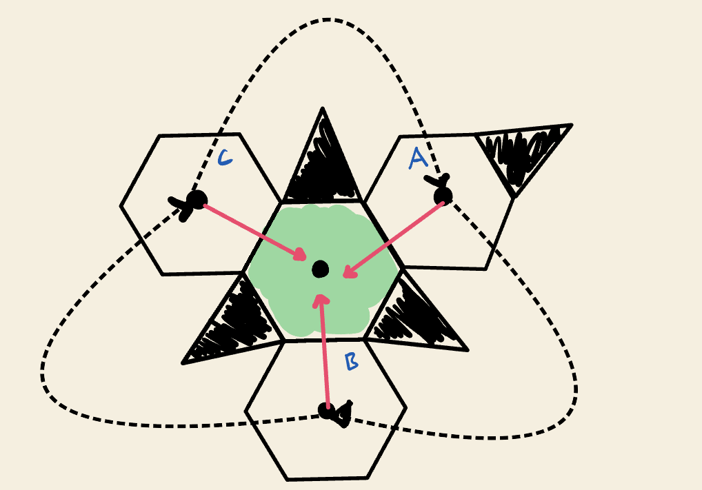
     <figcaption style="text-align: center; font-style: italic; font-size: 0.9em; color: #666;"> Figure 1. The truncated tetrahedron $T$ unfolded into the plane, with Andy's home hexagon in green. The other three white hexagons all border home, and the lone black triangle at the top right is the one face that doesn't touch home. After Andy's first step to $A$, forward and backward moves (dashed) carry him around the cycle $A \to B \to C \to A$ while a right turn (red) from any of $A$, $B$, or $C$ takes him home. </figcaption>

</figure>

<p>WLOG, assume Andy starts on the green hexagon and then always moves to hexagon $A$ and then faces towards hexagon $B$.  Since we are given that</p>
<blockquote>
  <p>throughout his walk, Andy remembers the turns he’s taken</p>
</blockquote>

<p>we need to find a way to model his movements throughout the rest of his walk. Given that he starts at $A$ facing $B$, we can model his path in the following way. Andy can make 3 types of “move”:</p>
<ul>
  <li>Forward: This takes him along one of the black arrows in the diagram (e.g. $A \to B$)</li>
  <li>Backwards: He walks in <em>reverse</em> along the black arrow into his current hexagon (e.g. $B \to A$)</li>
  <li>Right: He turns right along one of the red arrows and returns home.</li>
</ul>

<p>All three moves are defined from Andy’s own perspective. After his first step, Andy keeps track of which way he is facing, so at every hexagon the three exits are: the edge in front of him, the edge on his right, and the remaining edge. When he moves <em>forward</em>, he walks through the edge he is facing and then turns to face the exit on his left. A <em>backward</em> move undoes a forward move: he steps back through the remaining edge and turns to face the hexagon he just left. Turning <em>right</em> takes him through the edge on his right. Since each move depends only on Andy’s heading and the order of the edges around him, his memory of his turns tells him exactly which moves he made, and with these three moves he can always work out where he is relative to the first hexagon he entered.</p>

<p>For Andy to follow a sequence of turns, $S$, in the hexagonal tiling $T’$ and <em>not</em> notice that he left $T$, it must be the case that <em>$S$ returns Andy home in $T$ exactly once, and on the last move.</em> If Andy ever takes a move that would have returned him home in $T$ (i.e., turning right) but doesn’t in $T’$, then he knows he is not on $T$.</p>

<p>What do moves look like in $T’$?</p>

<p>Again assume Andy steps to hexagon $A$ and faces $B$. His possible moves on $T’$ are shown in the figure below.</p>

<figure>

  <img src="/assets/img/blog_images/2026-10-07-andys-amble/andy_hexa_path.png" alt="Andy's moves on the hexagonal tiling" width="40%" style="display: block; margin: auto;" />
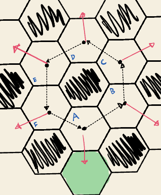
     <figcaption style="text-align: center; font-style: italic; font-size: 0.9em; color: #666;"> Figure 2. Andy's moves on the hexagonal tiling $T'$. Forward and backward moves keep him on the ring $A, B, \ldots, F$ around a black hexagon. A right turn (red) leads home only from $A$; from anywhere else it leads off the ring to a hexagon that isn't home. </figcaption>

</figure>

<p>Why does $T’$ look different? Locally, the two lands are identical: every white hexagon has three white neighbors spaced 120 degrees apart, so any sequence of turns can be replayed on either one. The only difference is the black tiles. A black triangle on $T$ is ringed by 3 white hexagons, while a black hexagon on $T’$ is ringed by 6. So the ring $A, B, \ldots, F$ wraps <em>twice</em> around the cycle $A, B, C$. For example, at $D$, Andy’s memory says he’s back at $A$.</p>

<p>This means that, unlike before, in $T’$, $A$ is the <em>only</em> position from which Andy can turn right and be in the home hexagon. The first time Andy turns right while not in hexagon $A$, he will notice he is not home and can tell he is in $T’$. Thus it now suffices to find the probability that the first time Andy turns right will be when he is in hexagon $A$.</p>

<p>We can set this up as a recurrence relationship (this is a random walk on a Markov chain). Let $p_i$ be the probability that Andy finishes his walk without noticing he is in $T’$, given he is currently in hexagon $i$, $i = A, B, \ldots, F$. From any hexagon on the ring, he moves forward, backward, or right, each with probability $\frac{1}{3}$. Turning right from $A$ takes him home undetected, while turning right from anywhere else gives him away. Reflecting the ring across the line through $A$ and $D$ gives the symmetries $p_B = p_F$ and $p_C = p_E$. We get the following system of equations</p>

\[\begin{aligned}
p_A &amp;= \frac{1}{3} + \frac{1}{3} p_B + \frac{1}{3} p_F = \frac{1}{3} + \frac{2}{3} p_B\\ 
p_B &amp; = \frac{1}{3} p_A + \frac{1}{3}p_C \\ 
p_C &amp; = \frac{1}{3} p_B + \frac{1}{3}p_D \\
p_D &amp; = \frac{1}{3} p_C + \frac{1}{3} p_E = \frac{2}{3}  p_C.
\end{aligned}\]

<p>A little algebra (or Mathematica 😅) later and we find, 
\(p_A = \frac{9}{20}.\)</p>

<p>However, note that this is the probability that Andy has a sequence of moves that <em>doesn’t</em> result in him finding out he is on $T’$. The puzzle asks for the complement, and thus our answer is 
\(\begin{equation*}
\boxed{p = 1- p_A = \frac{11}{20}}.
\end{equation*}\)</p>]]></content><author><name></name></author><category term="math" /><summary type="html"><![CDATA[My solution to the 2026 August Puzzle]]></summary></entry><entry><title type="html">Jane Street Puzzle: Planetary Parade</title><link href="https://ccolombe12.github.io/blog/2026/Planetary-Parade/" rel="alternate" type="text/html" title="Jane Street Puzzle: Planetary Parade" /><published>2026-04-01T00:00:01+00:00</published><updated>2026-04-01T00:00:01+00:00</updated><id>https://ccolombe12.github.io/blog/2026/Planetary-Parade</id><content type="html" xml:base="https://ccolombe12.github.io/blog/2026/Planetary-Parade/"><![CDATA[<h1 id="problem-statement">Problem Statement</h1>

<blockquote>
  <p>We are enjoying a planetary parade during the beginning of this month here on Earth, but my alien friend from the distant planet Pyrknot (well modeled as a perfect sphere) isn’t too impressed. Their single-star system has $n$ planets other than Pyrknot with such chaotic orbits that each night these planets independently appear in uniformly random locations in the Pyrknothian sky. Note that <em>the planets aren’t visible in daylight</em>. If at a given moment there exists somewhere on Pyrknot that all $n$ planets are visible, then from my friend’s position on the surface they have an $\alpha$ probability of also seeing all of the planets.</p>
</blockquote>

<blockquote>
  <p>My friend is considering building a tower to improve their chances of seeing these planetary parades (parade). Assume the tower allows the viewing of every celestial body that could be seen from at least one location on the surface of Pyrknot less than a distance $r$ from the base of the tower. In the limit of $r$ being small compared to the radius $R$ of Pyrknot, the new probability of seeing the planetary parade from the top of the tower is linearly approximated by $\alpha + \beta\cdot(r/R)$. <strong>Find $\alpha$ and $\beta$ in exact terms</strong>.</p>
</blockquote>

<hr />
<h1 id="solution">Solution</h1>

<p>We will solve this problem in a few parts, looking at the 2D and 3D versions of the problem. First, we will solve for $\alpha$, which turns out to be dimension-agnostic. Next, we will solve the problem in 2D (that is, for a circular planet whose universe is the plane) to build some intuition. Then, we will use our findings from the 2D case to construct the answer to the 3D version.</p>

<hr />

<h2 id="part-1-finding-alpha--a-dimension-agnostic-result">Part 1: Finding $\alpha$ — a dimension-agnostic result</h2>
<p>The key quantity throughout is $\alpha$, the probability of seeing the parade without a tower, given that a parade is taking place somewhere on the planet.</p>

<p>To start, let’s assume that our friend’s location on the planet is at the North Pole (NP). Assume that for our modeling purposes the celestial bodies in the system (not including Pyrknot) lie on some other sphere that is very far from the planet. For our purposes, we can say that the position of a planet in the sky can be mapped to a position on the surface of Pyrknot by drawing a line between the planet and the center of Pyrknot. That way, we can model the positions of celestial bodies around Pyrknot as positions on the surface of Pyrknot.</p>

<p>Now, given that a parade exists, what must be true for it to be visible from the NP? We have two conditions that must be satisfied:</p>

<ul>
  <li>It is night time at the NP (otherwise the parade is not visible)</li>
  <li>All $n$ planets must be in the hemisphere centered at the NP.</li>
</ul>

<p>We need to find the probability that, at a given moment, we can see the parade from the NP given that one exists. Using Bayes’ theorem, we can write this as</p>

\[\begin{equation}\label{eq:Bayes}
\begin{aligned}
\alpha &amp; := \Pr[\text{Parade visible from NP}|\text{Parade exists}]\\
 &amp; = \frac{\Pr[\text{Parade exists}|\text{Parade visible from NP}] \cdot\Pr\left[\text{Parade visible from NP}\right]}{\Pr\left[\text{Parade exists}\right]}    \\ 
&amp; = \frac{1 \cdot \Pr\left[\text{Parade visible from NP}\right]}{\Pr\left[\text{Parade exists}\right]}.  \\
\end{aligned}
\end{equation}\]

<p>The middle factor simplifies to 1 because if the parade is visible from the NP, it certainly exists somewhere on the planet.</p>

<p>Thus, it suffices for us to find $\Pr\left[\text{Parade visible from NP}\right]$ and $\Pr\left[\text{Parade exists}\right]$.</p>

<p>To find the probability that in a given moment a parade on $n$ planets is visible from the north pole, we need all the planets to be in the northern hemisphere and the star to be in the <em>opposite hemisphere</em>. Since the positions of all $n$ planets and the star are independent and uniform, each planet lies in the northern hemisphere with probability $\frac{1}{2}$ and the star lies in the southern hemisphere (making it night at the NP) with probability $\frac{1}{2}$, giving
\(\begin{equation}
\Pr\left[\text{Parade visible from NP}\right] = \frac{1}{2^{n + 1}}. \label{eq:NP_visibility}
\end{equation}\)</p>

<p>It is a bit more nuanced to find the probability that a parade exists somewhere on the surface of the planet since there could be many places where the parade is visible. However, there exists a well-known result that can help us out: <a href="https://en.wikipedia.org/wiki/Wendel%27s_theorem">Wendel’s theorem</a>, which gives us the probability that $n+1$ points randomly placed on the surface of a $d$-dimensional sphere are contained within some shared hemisphere. To use it within the context of our problem, we create a pseudo-planet that is placed antipodal to the location of the star. That way, we can find the probability that the $n$ planets and the pseudo-planet all exist in some shared hemisphere, which is equivalent to all $n$ planets being visible from some point while the star is not.</p>

<p>Wendel’s theorem states that in dimension $d$ with $n + 1$ points, the probability those points all lie in some shared hemisphere is: 
\(\begin{equation}
\label{eq:parade_exists}
\begin{aligned}
\Pr\left[\text{Parade exists}\right] = \frac{2 \sum_{k = 0}^{d - 1} \binom{n}{k}}{2^{n + 1}}. 
\end{aligned}
\end{equation}\)</p>

<p>If we combine equations (\ref{eq:Bayes}), (\ref{eq:NP_visibility}), and (\ref{eq:parade_exists}), we find that</p>

<p>\(\begin{equation}
\label{eq:alpha}
\begin{aligned} 
\alpha &amp; = \frac{ \Pr\left[\text{Parade visible from NP}\right]}{\Pr\left[\text{Parade exists}\right]}\\ 
&amp; = \frac{\frac{1}{2^{n + 1}}}{\frac{2 \sum_{k = 0}^{d - 1} \binom{n}{k}}{2^{n + 1}}}\\ 
&amp; = \boxed{\frac{1}{2 \sum_{k = 0}^{d - 1} \binom{n}{k}}},
\end{aligned}
\end{equation}\)
which is the reciprocal of the number of regions created by $n + 1$ non-degenerate great circles on a sphere in $d$ dimensions!</p>

<p>Next, we will introduce the tower and solve for $\beta$ in the case of $d = 2$.</p>

<hr />

<h2 id="part-2-a-tower-on-a-planet-in-the-plane-universe">Part 2: A tower on a planet in the plane-universe</h2>

<p>We now construct a tower at the north pole that allows us to see any body that would otherwise be visible from some point within distance $r$ from the base of the tower. In the limit of $r \ll R$, this is essentially a small arc on the circular planet of arclength $2r$. How does this affect our chances of seeing a parade? On one hand, it gives us a greater likelihood of seeing more planets in the sky at a given moment, but on the other hand, it also gives us a greater chance of seeing the star during that moment, which would ruin the parade.</p>

<p>Suppose we are just isolating the effect for a single planet $P$. Given that we have our tower of effective radius $r$, what is the probability of seeing the planet from the tower?</p>

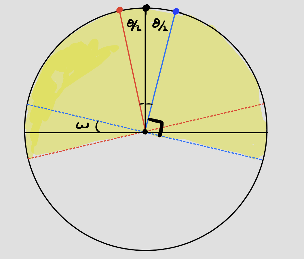
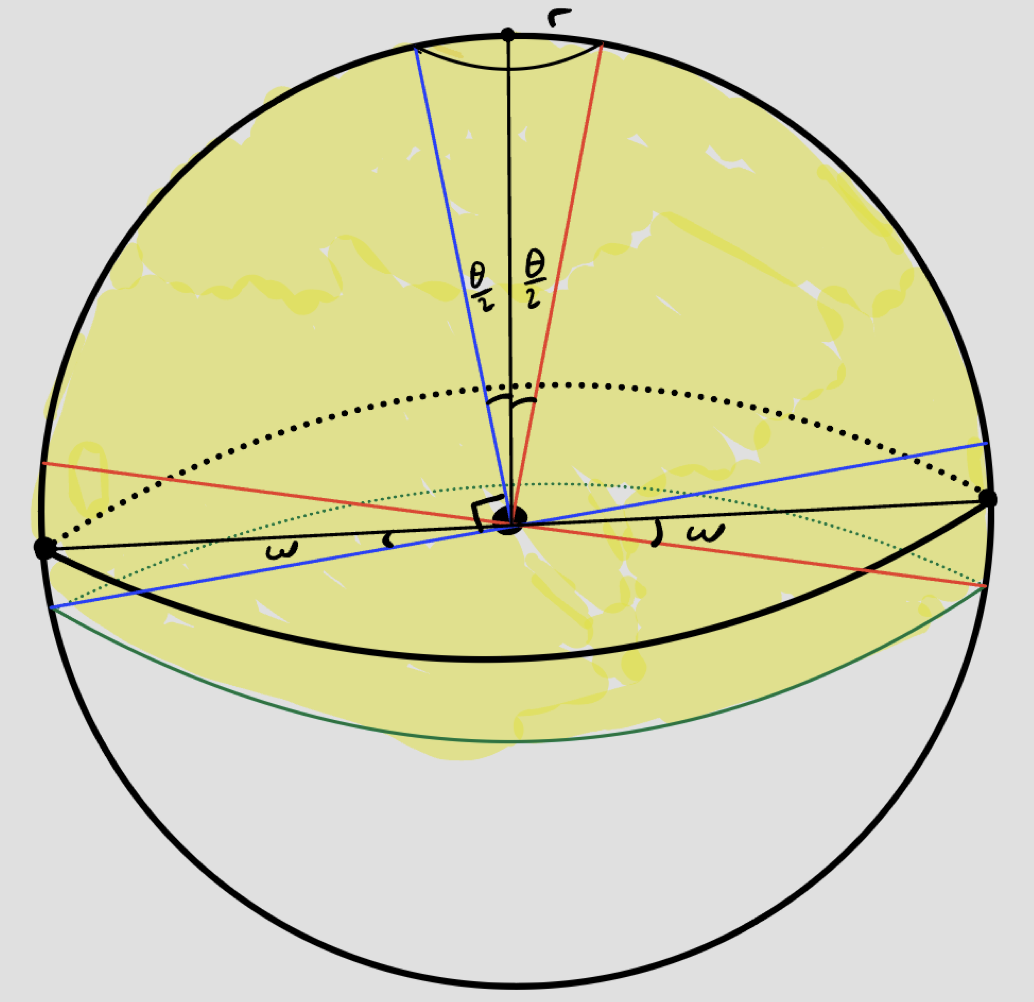
<p>Note that <em>without</em> the tower, the position of $P$ must lie above the equator. With the tower, we can now see all planets whose position dips slightly below the equator. Let $\theta$ be the angular diameter of the area that the tower can effectively view from. If we draw the diameters of the semicircles that are centered on the two edge points of our viewing region (red and blue points in Figure 1, respectively), we can see that the effective region in which planets are visible (yellow region in Figure 1) includes the northern hemisphere and two sectors of angle $\omega$ that dip below the equator.</p>

<figure>
  <center>
  <img src="/assets/img/blog_images/2026-04-01-planet-parade/pp-2d-case.png" width="60%" style="display: block; margin: auto;" />
     <figcaption style="text-align: center; font-style: italic; font-size: 0.9em; color: #666;"> Figure 1. The tower's effective viewing region in the 2D (circular planet) case. Without the tower, a planet must lie in the northern hemisphere to be visible. The tower extends this to the full yellow region, adding two sectors of angle $\omega = \theta/2$ below the equator, centered on the edge points of the base arc (shown in red and blue). </figcaption>
    </center>
</figure>

<p>Some elementary geometry yields that $\omega = \theta / 2$. Therefore, the fraction of the circle covered by the tower is $\frac{\pi + \theta}{2 \pi}$, and for a given planet, the probability that it is visible from the tower is:</p>

\[\begin{equation}
\Pr\left[\text{Planet $P$ visible from tower}\right] = \frac{1 + \theta/\pi}{2}. \label{eq:eff_area_2}
\end{equation}\]

<p>Now, for a parade to be visible from the tower, we need all $n$ planets to be visible and the star not to be.</p>

<p>Using the independence of the planets and the star along with (\ref{eq:eff_area_2}), we find</p>

\[\begin{equation*}
\begin{aligned}
\Pr\left[\text{Parade visible from tower}\right] &amp; = \left(\frac{1 + \theta/\pi}{2}\right)^n \left(\frac{1 - \theta/\pi}{2}\right)\\ 
&amp; = \frac{1}{2^{n+ 1}}(1 + \theta/\pi)^n (1 - \theta/\pi)\\
&amp; \approx \frac{1}{2^{n+ 1}}(1 + n\theta/\pi) (1 - \theta/\pi) &amp;&amp; (\text{apply binomial approx. for small $\theta$})\\
&amp; = \frac{1}{2^{n+ 1}}\left(1 + (n - 1)\theta/\pi - \mathcal{O}(\theta^2)\right)\\
&amp; \approx \frac{1}{2^{n+ 1}}(1 + (n - 1)\theta/\pi). &amp;&amp; (\text{drop higher order dependence})
\end{aligned}
\end{equation*}\]

<p>If we note that $\theta = 2r/R$ and use our previous expressions for the conditional probability (\ref{eq:Bayes}) and existence of a parade (\ref{eq:parade_exists}), we find:</p>

\[\begin{equation*}
\begin{aligned}
\Pr[\text{Parade visible from tower}|\text{Parade exists}] &amp; = \frac{\Pr\left[\text{Parade visible from tower}\right]}{\Pr\left[\text{Parade exists}\right]}\\
&amp; \approx \frac{\frac{1}{2^{n+ 1}}(1 + (n - 1)\theta/\pi)}{\frac{2 \sum_{k = 0}^{1} \binom{n}{k}}{2^{n + 1}}} \\
&amp; = \frac{1 + (n - 1)\theta/\pi}{2(n + 1)} &amp;&amp; \left(\text{since } \sum_{k=0}^{1}\tbinom{n}{k} = 1 + n\right)\\
&amp; = \frac{1}{2 (n + 1)} + \frac{n - 1}{2\pi(n + 1)} \cdot \theta\\
&amp; = \frac{1}{2 (n + 1)} + \frac{n - 1}{2\pi(n + 1)} \cdot \left(\frac{2r}{R}\right)\\ 
&amp; = \frac{1}{2 (n + 1)} + \frac{n - 1}{\pi(n + 1)} \cdot \left(\frac{r}{R}\right), \\ 
\end{aligned}
\end{equation*}\]

<p>which implies for $d = 2$, we find
\(\begin{equation*}
\boxed{
\begin{aligned}
\alpha &amp; = \frac{1}{2 (n + 1)}\\
\beta &amp; = \frac{n - 1}{\pi(n + 1)}.\\
\end{aligned}}
\end{equation*}\)</p>

<hr />

<h2 id="part-3-a-parade-on-the-sphere">Part 3: A Parade on the sphere</h2>

<p>Since (\ref{eq:alpha}) was derived for arbitrary $d$, it applies directly to the 3D case — we need only find $\beta$. In 3D the effective viewing area for the tower is now a small cap of the sphere of angular diameter $\theta$, which is again given by $\theta = 2r / R$. Now, the tower, instead of extending the total observable area by two arcs of angle $\theta/2$, adds an additional ring of area below the equator, shown between the thick black equator and the green circle in Figure 2.</p>

<figure>
  <center>
  <img src="/assets/img/blog_images/2026-04-01-planet-parade/pp-3d-case.png" width="60%" style="display: block; margin: auto;" />
     <figcaption style="text-align: center; font-style: italic; font-size: 0.9em; color: #666;"> Figure 2. The tower's effective viewing region in the 3D (sphere) case. Rather than two sectors, the tower adds an annular band of surface area $2\pi R^2 \sin(\theta/2)$ below the equator (yellow region, bounded below by the green circle), which increases the probability that any given planet is visible from the tower. </figcaption>
    </center>
</figure>

<p>To get the total observable area of the planet from the tower, we need to find the area $A(\theta)$ of the added ring.</p>

<p>Using spherical coordinates (with $\phi$ the polar angle measured from the north pole and $\lambda$ the azimuthal angle), we can write this surface area as:</p>

\[\begin{equation*}
\begin{aligned}
A(\theta) &amp; =\int_{0}^{2 \pi}\int^{\pi/2}_{\pi/2 - \theta/2} R^2\sin \phi \, d \phi \, d\lambda \\
&amp; = 2 \pi R^2 \sin(\theta/2).
\end{aligned}
\end{equation*}\]

<p>Therefore, the total area of the planet viewable from the tower is $2 \pi R^2 + 2 \pi R^2 \sin(\theta/2)$ and thus the probability of viewing any given planet is</p>

\[\Pr\left[\text{Planet $P$ visible from tower}\right] = \frac{2 \pi R^2 + 2 \pi R^2 \sin(\theta/2)}{4 \pi R^2} = \frac{1 + \sin(\theta/2)}{2}.\]

<p>Now all that remains is to find the probability that all planets are visible from the tower and the star is not. Using the same approach as in the 2D case, we find:</p>

\[\begin{equation}
\label{eq:tower_prob_3d}
\begin{aligned}
\Pr\left[\text{Parade visible from tower}\right] &amp; = \left(\frac{1 + \sin(\theta/2)}{2}\right)^n \left(\frac{1 - \sin(\theta/2)}{2}\right)\\ 
&amp; = \frac{1}{2^{n + 1}}\bigl(1 + \sin(\theta/2)\bigr)^n \bigl(1 - \sin(\theta/2)\bigr)\\
&amp; \approx \frac{1}{2^{n+ 1}}\bigl(1 + n\sin(\theta/2)\bigr) \bigl(1 - \sin(\theta/2)\bigr) &amp;&amp; (\text{binomial approx. for small $\theta$})\\
&amp; \approx \frac{1}{2^{n+ 1}}\bigl(1 + n\theta/2\bigr) \bigl(1 - \theta/2\bigr) &amp;&amp; (\text{small angle approx. for $\sin$})\\
&amp; = \frac{1}{2^{n+ 1}}\left(1 + (n - 1)\frac{\theta}{2} - \mathcal{O}(\theta ^2)\right)\\
&amp; \approx \frac{1}{2^{n+ 1}}\left(1 + (n - 1)\frac{\theta}{2}\right). &amp;&amp; (\text{drop higher order dependence})\\
\end{aligned}
\end{equation}\]

<p>Once again noting that $\theta = 2r/R$, and plugging (\ref{eq:parade_exists}) and (\ref{eq:tower_prob_3d}) into (\ref{eq:Bayes}), we find:</p>

\[\begin{equation*}
\begin{aligned}
\Pr[\text{Parade visible from tower}|\text{Parade exists}] &amp; = \frac{\Pr\left[\text{Parade visible from tower}\right]}{\Pr\left[\text{Parade exists}\right]}\\
&amp; \approx \frac{\frac{1}{2^{n+ 1}}\left(1 + (n - 1)\frac{\theta}{2}\right) }{\frac{2 \sum_{k = 0}^{2} \binom{n}{k}}{2^{n + 1}}} \\
&amp; = \frac{1 + (n - 1)\frac{\theta}{2}}{n^2 + n + 2} &amp;&amp; \left( 2\sum_{k=0}^{2}\tbinom{n}{k} = n^2+n+2\right)\\
&amp; =\frac{1 + (n - 1)\frac{r}{R}}{n^2 + n + 2} \\
&amp; = \frac{1}{n^2 + n + 2} + \frac{n - 1}{n^2 + n + 2}\cdot \left(\frac{r}{R}\right),
\end{aligned}
\end{equation*}\]

<p>which gives us our final answer:</p>

\[\begin{equation*}
\boxed{
\begin{aligned}
\alpha &amp; = \frac{1}{n^2 + n + 2}\\
\beta &amp; = \frac{n - 1}{n^2 + n + 2}.\\
\end{aligned}}
\end{equation*}\]

<hr />

<h2 id="remarks">Remarks</h2>

<p><strong>The tower is useless for $n = 1$.</strong> In both 2D and 3D, $\beta = 0$ when $n = 1$. The intuition is symmetric: for every configuration where the tower’s wider field of view lets you catch the single planet below the equator, there is an equally likely configuration where it causes you to see the star instead. These two effects cancel exactly at first order, so the tower provides no benefit.</p>

<p><strong>The tower always helps when $n &gt; 1$.</strong> For $n &gt; 1$, $\beta &gt; 0$ in both dimensions, meaning the tower strictly improves your odds. Intuitively, the tower’s extended range creates $n$ new opportunities to gain (one per planet) but only one opportunity to lose (the star). When $n &gt; 1$, the planets win on average.</p>

<p><strong>$\alpha$ decays much faster in 3D.</strong> For large $n$,</p>

\[\alpha_{2D} \approx \frac{1}{2n}, \qquad \alpha_{3D} \approx \frac{1}{n^2}.\]

<p>In 3D, there is so much more room in the sky that simultaneously fitting all $n$ planets into a hemisphere becomes quadratically harder. This reflects the general Wendel’s theorem result: higher-dimensional spheres make hemispheric coincidences exponentially rarer.</p>

<p><strong>The tower’s marginal benefit $\beta$ has different large-$n$ behavior by dimension.</strong> As $n \to \infty$,</p>

\[\beta_{2D} \to \frac{1}{\pi}, \qquad \beta_{3D} \to 0.\]

<p>In 2D, the marginal gain per unit $r/R$ converges to a positive constant. Even with very many planets, the tower always helps at first order. In 3D, the parade itself becomes so rare that even the tower’s extended range can’t keep up.</p>]]></content><author><name></name></author><category term="math" /><summary type="html"><![CDATA[My solution to the 2026 March Puzzle]]></summary></entry><entry><title type="html">Jane Street Puzzle: Robot Javelin</title><link href="https://ccolombe12.github.io/blog/2025/JS_Robot_Javelin/" rel="alternate" type="text/html" title="Jane Street Puzzle: Robot Javelin" /><published>2025-12-30T00:00:01+00:00</published><updated>2025-12-30T00:00:01+00:00</updated><id>https://ccolombe12.github.io/blog/2025/JS_Robot_Javelin</id><content type="html" xml:base="https://ccolombe12.github.io/blog/2025/JS_Robot_Javelin/"><![CDATA[<h1 id="problem-statement">Problem Statement</h1>

<blockquote>
  <p>It’s coming to the end of the year, which can only mean one thing: time for this year’s Robot Javelin finals! Whoa wait, you’ve never heard of Robot Javelin? Well then! Allow me to explain the rules:</p>
  <ul>
    <li>It’s head-to-head. Each of two robots makes their first throw, whose distance is a real number drawn uniformly from $[0, 1]$.</li>
    <li>Then, without knowledge of their competitor’s result, each robot decides whether to keep their current distance or erase it and go for a second throw, whose distance they must keep (it is also drawn uniformly from $[0, 1]$).</li>
    <li>The robot with the larger final distance wins.</li>
  </ul>
</blockquote>

<blockquote>
  <p>This year’s finals pits your robot, Java-lin ($J$), against the challenger, Spears Robot ($S$). Now, robots have been competing honorably for years and have settled into the Nash equilibrium for this game. However, you have just learned that Spears Robot has found and exploited a leak in the protocol of the game. They can receive a single bit of information telling them whether their opponent’s first throw (distance) was above or below some threshold $d$ of their choosing before deciding whether to go for a second throw. Spears has presumably chosen d to maximize their chance of winning — no wonder they made it to the finals!</p>
</blockquote>

<blockquote>
  <p>Spears Robot isn’t aware that you’ve learned this fact; they assume Java-lin is using the Nash equilibrium strategy.. <strong>If you were to adjust Java-lin’s strategy to maximize its odds of winning given this, what would be Java-lin’s updated probability of winning?</strong></p>
</blockquote>

<hr />
<h1 id="solution">Solution</h1>

<p>This problem naturally has three components:</p>

<ul>
  <li>What is the Nash equilibrium strategy in the vanilla game?</li>
  <li>Given that $S$ can see if $J$’s throw was more or less than $d$, what is their optimal $d^*$?</li>
  <li>Knowing that $S$ will play optimally with their new information but doesn’t know $J$ is aware of $S$’s strategy, what is the optimal strategy for $J$ now?</li>
</ul>

<h2 id="part-1-vanilla-nash-equilibrium">Part 1: Vanilla Nash Equilibrium</h2>

<p>We assume both robots use a threshold strategy and by symmetry they adopt the same threshold $\tau$. That is, both robots throw their first javelin. If they throw it further than distance $\tau$ then they keep their first throw, otherwise they throw again. In this first part, we’ll find the value of $\tau$.</p>

<p>Recall that in a Nash equilibrium, no player can unilaterally change their strategy and improve their position. So without loss of generality, let’s assume that $J$ uses $\tau$ and $S$ uses $t$. We would like to find the value of $\tau$ such that for all $t \in [0, 1]$, $S$’s probability of winning is maximized at $t = \tau$.</p>

<p>To do this, we first need an expression for the probability that $S$ wins given they use strategy $t$ and $J$ uses strategy $\tau$. Let $\tilde{s}$ and $\tilde{j}$ be random variables denoting the distance $S$ and $J$ use in their score respectively. We want to determine $\Pr[\tilde{s} &gt; \tilde{j}]$. We can write down the CDF of $\tilde{s}$ for fixed $t$ as:</p>

\[\begin{equation*}
F_S(s, t) = \begin{cases}
 t s &amp; 0\leq s\leq t \\
 (s-t) + s t &amp; t&lt;s&lt;1.
\end{cases}
\end{equation*}\]

<p>This follows from the fact that the only way to throw at most $s$ for $s \leq t$ is to throw under $t$ the first throw, then under $s$ the second. And for $s &gt; t$ we can throw between it and $t$ on our first throw with probability $s - t$ or below $t$ on the first throw and then under $s$ the second. By the same logic, the CDF of $\tilde{j}$ is</p>

\[\begin{equation*}
F_J(j) = \begin{cases}
 \tau j &amp; 0\leq j\leq \tau \\
 (j-\tau) + j \tau &amp; \tau&lt;j&lt;1.
\end{cases}
\end{equation*}\]

<p>With these, we can write  $\Pr[\tilde{s} &gt; \tilde{j}]$ as a function of $t$.</p>

\[\begin{equation}
\begin{aligned}
\Pr\left[\tilde{s} &gt; \tilde{j}\right](t, \tau) &amp; = \int_{0}^1 F_J(s) f_s(s, t) \; ds \\
&amp; = \begin{cases}
 \frac{1}{2} \left(\tau ^2-\tau -\tau  t^2+\left(\tau ^2-\tau +1\right) t+1\right) &amp; 0\leq t \leq \tau \\
\frac{1}{2} \left(-\tau -\left((\tau +1) t^2\right)+\left(\tau ^2+\tau +1\right) t+1\right) &amp; \tau&lt;t&lt;1.
\end{cases}
\end{aligned}\label{eq:van_nash}
\end{equation}\]

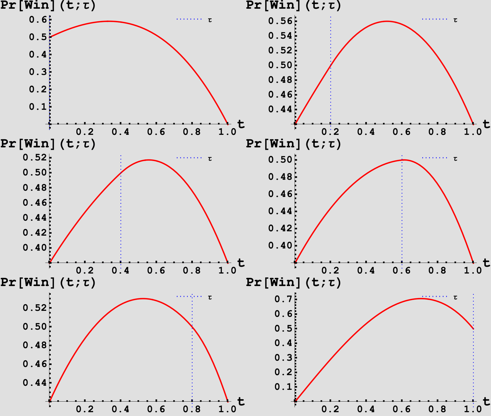
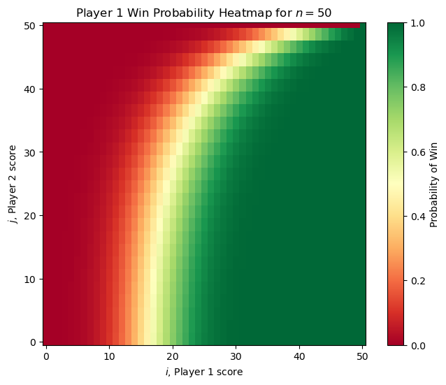
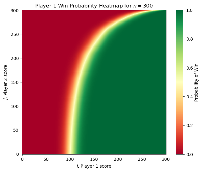
<p>Now, we would like to find the value of $\tau$ such that:  $\Pr \left[\tilde{s} &gt; \tilde{j}\right](t, \tau)$ is maximized in $t$ at $t = \tau$. If we vary $\tau$ and plot the probability of winning as a function of $t$, we can see that there is some $\tau$ for which the function in $t$ is strictly <em>decreasing</em> in $t$ on either side of $t = \tau$.</p>

<figure>
  <center>
  <img src="/assets/img/blog_images/2026-01-01-robot-javelin/P1_tau_animation.gif" width="60%" style="display: block; margin: auto;" />
     <figcaption style="text-align: center;"> Figure 1. As we vary $\tau$, we see that the plot of Probability of winning as a function of $t$ is maximized at $t = \tau$ when $\tau \approx 0.6$.  </figcaption>
    </center>
</figure>

<p>Taking the derivative of (\ref{eq:van_nash}) in $t$, setting $t = \tau$, and then solving for the root in $\tau$ yields a value of</p>

\[\begin{equation*}
\boxed{\tau = \frac{\sqrt{5} - 1}{2}}
\end{equation*}\]

<p>which is the unique Nash-equilibrium threshold strategy in the vanilla game and aligns with the value we would expect from Figure 1.</p>

<h2 id="part-2-optimal-cheating">Part 2: Optimal Cheating</h2>

<p>The next step is to determine what value of $d$ player $S$ should use to cheat in an optimal way. Recall that $S$ is choosing $d$ with the belief that $J$ is using the vanilla strategy with threshold $\tau$.</p>

<p>To choose $d$, $S$ can utilize two pieces of information: their initial throw value and a bit indicating whether or not $J$’s first throw exceeded $d$. From this information, $S$ must decide to <code class="language-plaintext highlighter-rouge">rethrow</code> or <code class="language-plaintext highlighter-rouge">keep</code>. Like in the previous section, we will develop an expression for the probability $S$ wins when $d \leq \tau$ and $d &gt; \tau$ and use those to determine an optimal value for $d$.</p>
<h3 id="case-1-d--tau">Case 1: $d &lt; \tau$</h3>
<p>Suppose $d \leq \tau$ and $S$’s initial throw was $s_1$. We can break up the probability $S$ wins by considering the cases where $J$’s first throw, denoted $j_1$, was more or less than $d$. If $j_1 &lt; d \leq \tau$, then $S$ knows that $J$ will <code class="language-plaintext highlighter-rouge">rethrow</code>. In that case, $S$ will <code class="language-plaintext highlighter-rouge">keep</code> if their initial throw was at least $1/2$ and <code class="language-plaintext highlighter-rouge">rethrow</code> otherwise. Therefore, the probability of $S$ winning if they initially throw $s$ and observe that $j_1 &lt; d$ is $P_{lo}(s_1) = \max(s_1, 1/2)$ where the first term represents keeping their initial throw of $s$ and the second is the event they both <code class="language-plaintext highlighter-rouge">rethrow</code>.</p>

<p>On the other hand, if $j_1 &gt; d$ then since $d \leq \tau$, $J$ may <code class="language-plaintext highlighter-rouge">rethrow</code> or <code class="language-plaintext highlighter-rouge">keep</code>. If $S$ <code class="language-plaintext highlighter-rouge">keeps</code> here, they win with probability</p>

\[\begin{equation*}P_{keep}(s_1) = \underbrace{\max \left\{0,\frac{s_1 -\tau }{1-\tau }\right\}\frac{1-\tau }{1-d} }_{\text{$J$ keeps, $S$ keeps}} + \underbrace{ s_1\frac{(\tau -d)}{1-d}}_{\text{$J$ rethrows, $S$ keeps}}.
\end{equation*}\]

<p>By the same conditioning logic, we find that if $S$ <code class="language-plaintext highlighter-rouge">rethrows</code> they win with probability</p>

\[\begin{equation*}P_{throw} = \underbrace{\frac{1-\tau }{2}\frac{1-\tau}{1-d}}_{\text{$J$ keeps, $S$ rethrows}} + \underbrace{\frac{1}{2}\frac{\tau  - d}{1-d}}_{\text{$J$ rethrows, $S$ rethrows}}.
\end{equation*}\]

<p>$S$ will choose the larger of $P_{keep}(s_1)$ and $P_{throw}$ depending on the value of $s_1$.</p>

<p>Putting it together and integrating these cases over the possible values of $s_1$, the probability of $S$ winning for a given $d \leq \tau$ is</p>

\[\begin{equation*}
\begin{aligned}
P_{Win (d &lt; \tau)}(d) &amp; = \int_{0}^1\bigg( d \cdot P_{lo}(s_1) + (1 - d)\cdot \max\bigg\{P_{keep}(s_1), P_{throw} \bigg\}\bigg) \; d s_1 \\
                   &amp; = \frac{\left(19-5 \sqrt{5}\right) d^2-\left(11 \sqrt{5}+1\right) d+4 \left(\sqrt{5}+3\right)}{4 \left(-2 d+\sqrt{5}+1\right)^2}
\end{aligned}
\end{equation*}\]

<h4 id="case-2-d--tau">Case 2: $d &gt; \tau$</h4>
<p>Now, we must perform the same analysis for $d &gt; \tau$. If $S$ observes that $j_1 \geq d \geq \tau$, then they will know $J$ will <code class="language-plaintext highlighter-rouge">keep</code> with certainty. If $S$ <code class="language-plaintext highlighter-rouge">rethrows</code> they win with probability $(1 - d)/2$, and if they <code class="language-plaintext highlighter-rouge">keep</code>, they win with probability $\max ( 0, (s_1 - d)/(1 - d) )$. Putting these together, in the event that $S$ observes that $J$ throws more than $d$, $S$ wins with probability</p>

\[\begin{equation*}
P_{hi}(s_1) = \max\bigg\{\frac{1 - d}{2}, \frac{s_1 - d}{1 - d}\bigg\}
\end{equation*}\]

<p>Next, in the event $S$ observes $j_1 &lt; d$,  $J$ may <code class="language-plaintext highlighter-rouge">rethrow</code> or <code class="language-plaintext highlighter-rouge">keep</code>, so we need to use the same conditioning logic as in the previous case. Doing so, we find that the probability of $S$ winning when they <code class="language-plaintext highlighter-rouge">keep</code> and <code class="language-plaintext highlighter-rouge">rethrow</code> are:</p>

\[\begin{equation*}
P_{keep}(s_1) = \begin{cases}
\frac{\tau}{d} s_1 &amp; 0 \leq s_1 \leq \tau \\
\frac{\tau}{d} s_1  + \frac{s_1 - \tau}{s_1} &amp; \tau &lt; s_1 \leq d \\
\frac{\tau }{d} s_1 + 1 -\frac{\tau }{d} &amp; s_1 &gt; d \\
\end{cases} 
\end{equation*}\]

\[\begin{equation*}P_{throw} = 1 - \underbrace{\frac{(d-\tau ) (d+\tau )}{2 d}}_{\text{$J$ keeps, $S$ rethrows}}- \underbrace{\frac{\tau }{2 d}}_{\text{$J$ keeps, $S$ rethrows}}
\end{equation*}.\]

<p>As for a brief explanation of the terms in $P_{keep}(s_1)$, note since $j_1 &lt; d$, $J$ will rethrow with probability $d/\tau$ and then the second throw will be less than $s_1$ with probability $s_1$. That is why the term $\tau s_1/d $ appears in each case. The last two terms consider the additional case where $J$ <code class="language-plaintext highlighter-rouge">keeps</code>. For the middle term, some $j_1$ can beat $s_1$ in this interval; whereas in the last term, since $s_1 &gt; d &gt; j_1$, $S$ wins.</p>

<p>Similar to in the previous case, $S$ will choose the larger of the two options $P_{keep}(s_1)$ and $P_{throw}$. We can now integrate the probability of winning when $d &gt; \tau$ as a function of $s$ to get
\(\begin{equation*}
\begin{aligned}
P_{Win (d &gt; \tau)}(d) &amp; = \int_{0}^1\bigg( d \cdot P_{hi}(s_1) + (1 - d) \cdot \max\bigg\{P_{keep}(s_1), P_{throw} \bigg\} \bigg)\;ds_1 \\
                   &amp; = \frac{\left(\sqrt{5}+1\right) d^4-8 d^3+2 \left(\sqrt{5}+1\right) d^2-8 \left(\sqrt{5}-2\right) d+9 \sqrt{5}-15}{8 \left(\sqrt{5}-1\right)}
\end{aligned}
\end{equation*}\)</p>

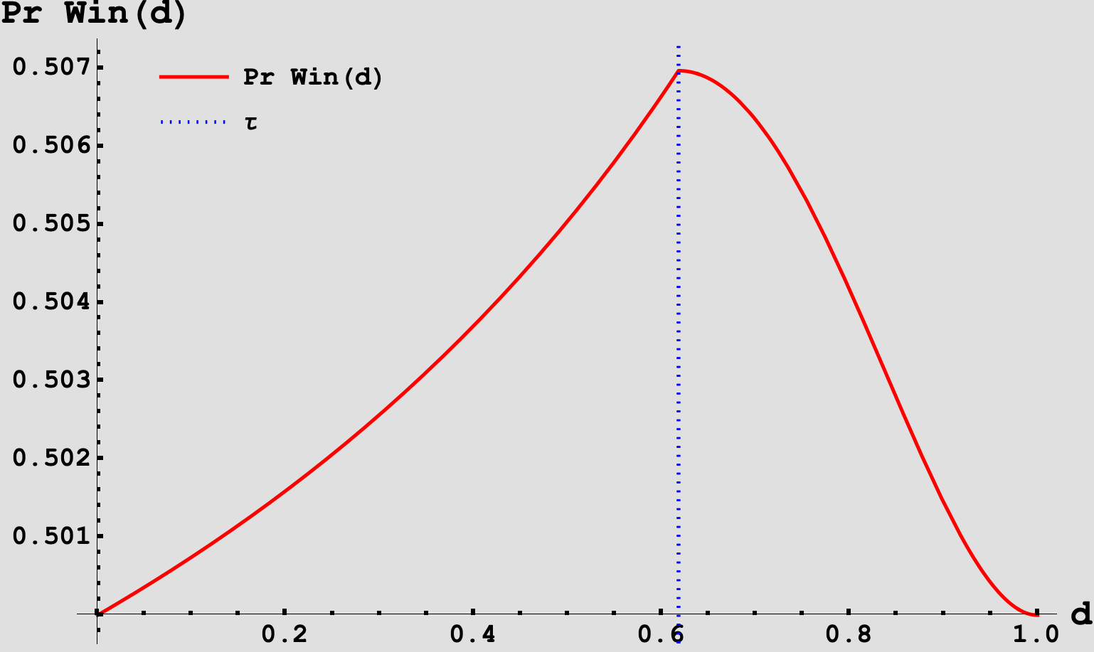
<p>If we now plot the probability of $S$ winning as a piecewise function in $d$ consisting of $P_{Win (d &lt; \tau)}(d)$ and $P_{Win (d &gt; \tau)}(d)$, we see:</p>

<figure>
  <center>
  <img src="/assets/img/blog_images/2026-01-01-robot-javelin/PrWin_d.png" width="60%" style="display: block; margin: auto;" />
     <figcaption style="text-align: center;"> Figure 2. Plot of the probability of $S$ of winning under optimal play as a function of $d$, the value they can query.  </figcaption>
    </center>
</figure>

<p>this implies that $\boxed{d^* = \tau}$. We can then further verify this by noting that the derivatives of $P_{Win (d &lt; \tau)}(d)$ and $P_{Win (d &gt; \tau)}(d)$ are strictly increasing and decreasing in $d$ for their respective regions.</p>

<p>The takeaway is that the optimal query is simply whether $J$ will rethrow. When $S$ does this, they win with probability</p>

\[\Pr[S \text{ win}](d^*) = \frac{1}{8} \left(13-4 \sqrt{5}\right) \approx 0.506966.\]

<p>Which is a slight edge above the previous 50-50 outcome.</p>

<h2 id="part-3-js-optimal-response-to-cheating">Part 3: $J$’s Optimal Response to Cheating</h2>

<p>Lastly, $J$ knows that $S$ can tell if $J$’s first throw is below or above $\tau$. How can $J$ use this information to devise an optimal response to $S$’s cheating? $S$’s behavior will vary depending on whether or not $J$’s first throw was more or less than $\tau$. We can assume $J$ uses a threshold strategy that depends on the first throw. Let $r$ be the new threshold used by $J$.</p>

<p>First suppose that  $j_1 \leq \tau$ . When should $J$ keep the first throw?</p>

<p>Since $S$ is cheating, they know $j_1 \leq \tau$. Based on the strategy we discovered in the previous part the CDF of the final value $S$ receives is</p>

\[\begin{equation*}
F_S(s) = \begin{cases}
 \frac{s}{2} &amp; 0\leq s \leq \frac{1}{2} \\
 \frac{3 s}{2}-\frac{1}{2} &amp; \frac{1}{2}\leq s \leq 1 .
\end{cases}
\end{equation*}\]

<p>For fixed threshold $r &lt; \tau$ we can develop the corresponding CDF and PDF for $J$’s final value</p>

\[\begin{equation*}
F_J(j, r) = \begin{cases}
 \frac{r j}{\tau } &amp; 0\leq j\leq r \\
 \frac{r j}{\tau } + \frac{j-r}{\tau } &amp; r\leq j\leq \tau  \\
 \frac{r j}{\tau } + 1 - \frac{r}{\tau} &amp; \tau \leq j\leq 1 \\
\end{cases}
\end{equation*}\]

\[\begin{equation*}
f_J(j, r) = \begin{cases}
 \frac{r}{\tau } &amp; 0\leq j\leq r \\
 \frac{r + 1}{\tau } &amp; r\leq j\leq \tau  \\
 \frac{r}{\tau } &amp; \tau \leq j\leq 1 \\
\end{cases}.
\end{equation*}\]

<p>Thus, the probability of $J$ winning as a function of $r$ is</p>

\[\begin{equation*}
\Pr\left[ J \text{ win}| j_1 \leq \tau\right](r) = \int_0^1 F_S(j) \cdot f_J(j) \;dj. 
\end{equation*}\]

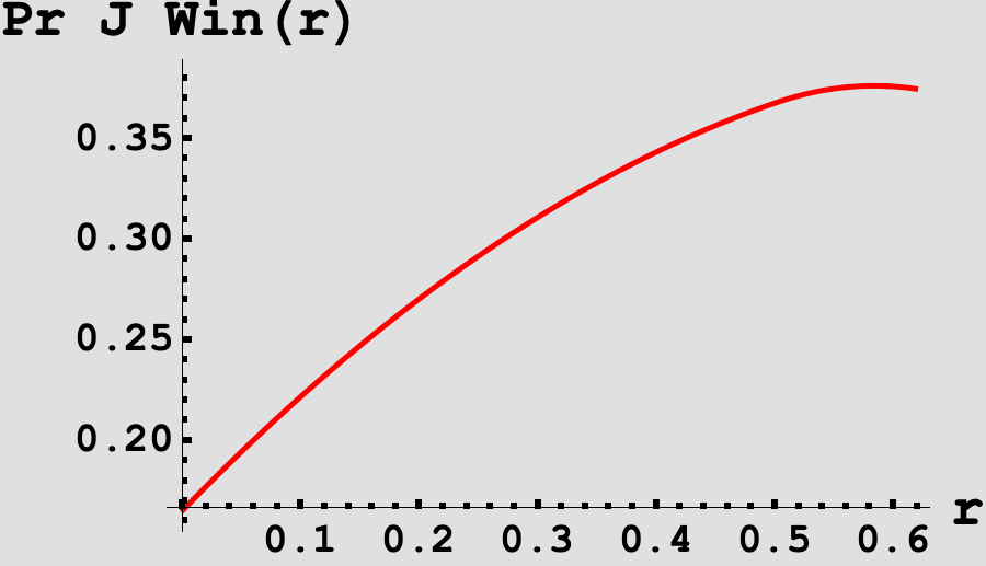
<p>We visualize this below in Figure 3.</p>
<figure>
  <center>
  <img src="/assets/img/blog_images/2026-01-01-robot-javelin/rThresh.png" width="60%" style="display: block; margin: auto;" />
     <figcaption style="text-align: center;"> Figure 3. The probability of $J$ winning using response threshold $r$ when $j_1 \leq \tau$.  </figcaption>
    </center>
</figure>

<p>From the figure, we see that the function seems to be unimodal with a maximum somewhere just before the threshold. Sure enough, if we take the derivative and solve for the root, we find that $\boxed{r^* = 7/12}$ is the optimal threshold strategy for $J$ when $j_1 \leq \tau$ which yields</p>

\[\begin{equation*}
\Pr\left[J \text{ win}| j_1 \leq \tau\right](r^*)  =\frac{\frac{313}{24}-5 \sqrt{5}}{4 \left(\sqrt{5} - 1\right)}.
\end{equation*}\]

<p>In summary, there is now a window, $[7/12, \tau]$, such that when $J$’s first throw falls in this window, $J$ can take advantage of $S$’s cheating and <code class="language-plaintext highlighter-rouge">keep</code> when $S$ thinks that $J$ will <code class="language-plaintext highlighter-rouge">rethrow</code>.</p>

<p>In the event that $j_1 &gt; \tau$, we can suppose another threshold $r’$ and repeat the same steps as before. However, this time we find that $\Pr\left[J \text{ win}\mid j_1 &gt; \tau\right](r’)$ is a strictly decreasing function for $r’ \geq \tau$, implying that when $J$’s first throw exceeds $\tau$, they should always <code class="language-plaintext highlighter-rouge">keep</code>, as in the vanilla strategy. Furthermore, when plugging in $r’ = \tau$, we find that</p>

\[\begin{equation*}
\Pr\left[J \text{ win}| j_1 &gt; \tau\right](\tau)  =\frac{1}{8} \left(2 \sqrt{5}+1\right).
\end{equation*}\]

<p>We have now worked out everyone’s optimal strategy and now it remains to compute the probability that $J$ wins! By conditioning on the event that $J$’s first throw is below or above $\tau$, we finally find</p>

\[\begin{equation*}
\begin{aligned}
\Pr\left[J \text{ win}\right]  &amp; =  \Pr\left[J \text{ win}| j_1 \leq \tau\right](r^*) \cdot \Pr[j_1 \leq \tau] + \Pr\left[J  \text{ win}| j_1 &gt;  \tau\right](\tau) \cdot \Pr[j_1 &gt; \tau] \\
                &amp; = \frac{\frac{313}{24}-5 \sqrt{5}}{4 \left(\sqrt{5} - 1\right)} \cdot \tau + \frac{1}{8} \left(2 \sqrt{5}+1\right) \cdot (1 - \tau) \\ 
            &amp; = \boxed{\frac{1}{192} \left(229-60 \sqrt{5}\right)}\\
\end{aligned}
\end{equation*}\]

<p>How does this fare against the previous odds when $J$ did not know $S$ was cheating? Previously, against cheating $S$, $J$ won with probability $0.493034$ whereas now they win with probability $0.493937$. A <em>very</em> minor improvement. Unfortunately for $J$, $S$’s cheating is hard to recover from. Fortunately for them, the game is still nearly 50-50!</p>]]></content><author><name></name></author><category term="math" /><summary type="html"><![CDATA[My solution to the 2025 December Puzzle]]></summary></entry><entry><title type="html">Jane Street Puzzle: Robot Baseball</title><link href="https://ccolombe12.github.io/blog/2025/JS_baseball/" rel="alternate" type="text/html" title="Jane Street Puzzle: Robot Baseball" /><published>2025-11-01T00:00:01+00:00</published><updated>2025-11-01T00:00:01+00:00</updated><id>https://ccolombe12.github.io/blog/2025/JS_baseball</id><content type="html" xml:base="https://ccolombe12.github.io/blog/2025/JS_baseball/"><![CDATA[<h2 id="problem-statement">Problem Statement</h2>
<blockquote>
  <p>The Artificial Automaton Athletics Association (Quad-A) is at it again, to compete with postseason baseball they are developing a Robot Baseball competition. Games are composed of a series of independent at-bats in which the Batter is trying to <em>maximize expected score</em> and the Pitcher is trying to <em>minimize expected score</em>.</p>
</blockquote>

<blockquote>
  <p>An at-bat is a series of pitches with a running count of balls and strikes, both starting at zero. For each pitch, the Pitcher decides whether to throw a ball or strike, and the Batter decides whether to wait or swing; these decisions are made secretly and simultaneously. The results of these choices are as follows.</p>
  <ul>
    <li>If the Pitcher throws a ball and the Batter waits, the count of balls is incremented by $1$.</li>
    <li>If the Pitcher throws a strike and the Batter waits, the count of strikes is incremented by $1$.</li>
    <li>If the Pitcher throws a ball and the Batter swings, the count of strikes is incremented by $1$.</li>
    <li>If the Pitcher throws a strike and the Batter swings, with probability $p$ the Batter hits a home run and with probability $1-p$ the count of strikes is incremented by $1$.</li>
  </ul>
</blockquote>

<blockquote>
  <p>An at-bat ends when either:</p>
  <ul>
    <li>The count of balls reaches $4$, in which case the Batter receives $1$ point.</li>
    <li>The count of strikes reaches $3$, in which case the Batter receives $0$ points.</li>
    <li>The Batter hits a home run, in which case the Batter receives $4$ points.</li>
  </ul>
</blockquote>

<blockquote>
  <p>By varying the size of the strike zone, Quad-A can adjust the value $p$, the probability a pitched strike that is swung at results in a home run. They have found that viewers are most excited by at-bats that reach a full count, that is, the at-bats that reach the state of three balls and two strikes. Let $q$ be the probability of at-bats reaching full count; $q$ is dependent on p. Assume the Batter and Pitcher are both using optimal mixed strategies and Quad-A has chosen the $p$ that maximizes $q$. <strong>Find this $q$, the maximal probability at-bats reach full count, to ten decimal places</strong>.</p>
</blockquote>

<hr />
<h1 id="solution">Solution</h1>

<p>We can solve this problem by modeling it as finite-state Markov chain. Let the states be given by the set \(S = \left\{(b, s) : s \in \{0,\ldots,3\}, b \in \{0,\ldots,4\}\right\}\) where $(b, s)$ represents the state with $b$ balls and $s$ strikes. Depending on the decisions made by the pair of robots at a given state (<code class="language-plaintext highlighter-rouge">swing</code> or <code class="language-plaintext highlighter-rouge">wait</code> for the Batter and <code class="language-plaintext highlighter-rouge">strike</code> and <code class="language-plaintext highlighter-rouge">ball</code> for the Pitcher respectively), we transition to one of several possible states, each with their own transition probability.</p>

<p>If we knew the transition probabilities between all states as a function of $p$, then we can tune $p$ such that the probability of reaching a full count from the initial state $(0,0)$ is maximized. Thus we will approach the remainder of the problem in three steps:</p>

<ul>
  <li>For a given state $(b, s)$ determine the optimal strategies for each player.</li>
  <li>Given the optimal strategies, determine the transition probabilities between states in the induced Markov chain.</li>
  <li>Determine the probability of reaching a full count and then select $p$ as to maximize it.</li>
</ul>

<h3 id="optimal-strategies">Optimal Strategies</h3>
<p>Let $V(b, s)$ be the expected score of the Batter at state $(b, s)$. For a given state, we have a subgame where the Batter is trying to maximize the  expected score and the Pitcher to minimize it. What are the optimal strategies for this subgame?</p>

<p>We can describe the strategies of the players using the concept of mixed-strategies. Let $x \in [0,1]$ and $y \in [0, 1]$ be the probabilities that the Batter  plays <code class="language-plaintext highlighter-rouge">swing</code> and the Pitcher plays <code class="language-plaintext highlighter-rouge">strike</code> at state $(b,s)$ respectively. How can we determine what these two ought to be in an equilibrium strategy? Recall that in a <a href="https://en.wikipedia.org/wiki/Nash_equilibrium">Nash equilibrium</a>, neither player can increase their objective by altering their current strategy. By the nature of our game, we can reason that neither player should use a pure strategy, as the opponent (or the player) could then deviate and improve their payout (Think rock, paper, scissors here – If your opponent always plays <code class="language-plaintext highlighter-rouge">rock</code> you should drop whatever strategy you are using and play <code class="language-plaintext highlighter-rouge">paper</code>). So what does a mixed strategy equilibrium look like in this case, does one even exist?</p>

<p>It turns out that, yes, one does exist! Since the subgame has a finite number of players (two) and a finite number of pure strategies (two each), it famously follows that the game will indeed have <a href="https://en.wikipedia.org/wiki/Nash_equilibrium#Existence">at least one Nash equillibrium in mixed-strategies</a>. Now, can we find it?</p>

<p>Suppose that $(x, y)$ forms a mixed-strategy Nash equilibrium and that the Batter was considering changing $x$ in an attempt to increase their score. The expected payoff to the Batter using strategy $x$, for fixed $y$, is given by:</p>

\[\begin{equation}
\begin{aligned}
V(b, s | x) &amp; = x \underbrace{\bigg(y(4 p  + (1 - p) V(b, s + 1) ) + (1 - y) V(b, s + 1)\bigg)}_{\text{Expected score from SWING}} \\
&amp; \qquad + (1 - x)\underbrace{\bigg(y V(b, s + 1) + (1 - y) V(b + 1, s)\bigg)}_{\text{Expected score from WAIT}}.
\end{aligned}\label{eq:payoff1}
\end{equation}\]

<p>To determine their strategy $y$, the Pitcher should choose $y$ such that the Batter cannot do better by deviating from $x$. For <em>fixed</em> $y$, we can write (\ref{eq:payoff1}) as</p>

\[\begin{equation}
V(b, s | x)  = x C_1(y) + (1 - x) C_2(y) \label{eq:payoff2}
\end{equation}\]

<p>where $C_1(y), C_2(y)$ are constants that depend on $y$. Observe that (\ref{eq:payoff2}) is maximized at $x = 0$ when $C_1(y) &lt; C_2(y)$, $x = 1$ when $C_1(y) &gt; C_2(y)$, and any $x \in [0, 1]$ when $C_1 = C_2$. From this observation, it follows that if the Pitcher were to set $y$ such that $C_1(y) = C_2(y)$, then the Batter cannot improve their payoff by deviating from $x$.</p>

<p>We can solve for $y$ such that $C_1(y) = C_2(y)$. Doing so, we find that</p>

\[\begin{equation}
\boxed{y^*(b, s) = \frac{V(b + 1,s)-V(b,s + 1)}{V(b + 1,s) - V(b,s + 1) + p(4 - V(b,s+1))}}. \label{eq:y_strat}
\end{equation}\]

<p>From (\ref{eq:y_strat}), since for any $(b, s) \in S$, we have that $V(b, s) \leq 4$ and $V(b + 1,s) \geq V(b,s + 1)$, it follows that $y(b, s) \in [0,1]$, which implies $y$ is a well-defined probability value.</p>

<p>Now, since the Batter and Pitcher share the same objective function, but different optimization directions, we can apply the same logic to ensure that the Pitcher cannot improve their payoff by deviating from $y(b, s)$, to find the corresponding Nash equilibrium strategy of</p>

\[\begin{equation}
\boxed{x^*(b, s) = y^*(b, s) }. \label{eq:x_strat}
\end{equation}\]

<p>Now that we have found the unique Nash equilibrium strategy pair in this game <sup id="fnref:1"><a href="#fn:1" class="footnote" rel="footnote" role="doc-noteref">1</a></sup> . We need to apply backwards induction using our state payoffs $V$ to find the exact value of each $x(b, s)$.</p>

<p>As mentioned in the problem statement, the payout to the Batter for striking out is $0$, for getting a walk is $1$, and for hitting a Homerun is $4$. Therefore the payouts are $V(b, 3) = 0$, $V(4, s) = 1$. We can solve for the Batter score function under the equilibrium strategies using the Mathematica code below.</p>

<div class="language-mathematica highlighter-rouge"><div class="highlight"><pre class="highlight"><code><span class="nv">B</span><span class="w"> </span><span class="o">=</span><span class="w"> </span><span class="m">4</span><span class="o">;</span><span class="w">
</span><span class="nv">S</span><span class="w"> </span><span class="o">=</span><span class="w"> </span><span class="m">3</span><span class="o">;</span><span class="w">
</span><span class="c">(* Base Cases *)</span><span class="w">
</span><span class="nv">V</span><span class="p">[</span><span class="nv">b</span><span class="o">_</span><span class="w"> </span><span class="o">/;</span><span class="w"> </span><span class="nv">b</span><span class="w"> </span><span class="o">==</span><span class="w"> </span><span class="nv">B</span><span class="o">,</span><span class="w"> </span><span class="nv">s</span><span class="o">_</span><span class="p">]</span><span class="w"> </span><span class="o">:=</span><span class="w"> </span><span class="m">1</span><span class="w"> 
</span><span class="nv">V</span><span class="p">[</span><span class="nv">b</span><span class="o">_,</span><span class="w"> </span><span class="nv">s</span><span class="o">_</span><span class="w"> </span><span class="o">/;</span><span class="w"> </span><span class="nv">s</span><span class="w"> </span><span class="o">==</span><span class="w"> </span><span class="nv">S</span><span class="p">]</span><span class="w"> </span><span class="o">:=</span><span class="w"> </span><span class="m">0</span><span class="w">

</span><span class="c">(*Define equilibrium strategies*)</span><span class="w">
</span><span class="nv">x</span><span class="p">[</span><span class="nv">b</span><span class="o">_,</span><span class="w"> </span><span class="nv">s</span><span class="o">_</span><span class="p">]</span><span class="w"> </span><span class="o">:=</span><span class="w"> 
 </span><span class="nv">x</span><span class="p">[</span><span class="nv">b</span><span class="o">,</span><span class="w"> </span><span class="nv">s</span><span class="p">]</span><span class="w"> </span><span class="o">=</span><span class="w"> 
  </span><span class="nb">Simplify</span><span class="p">[(</span><span class="nv">V</span><span class="p">[</span><span class="nv">b</span><span class="w"> </span><span class="o">+</span><span class="w"> </span><span class="m">1</span><span class="o">,</span><span class="w"> </span><span class="nv">s</span><span class="p">]</span><span class="w"> </span><span class="o">-</span><span class="w"> </span><span class="nv">V</span><span class="p">[</span><span class="nv">b</span><span class="o">,</span><span class="w"> </span><span class="nv">s</span><span class="w"> </span><span class="o">+</span><span class="w"> </span><span class="m">1</span><span class="p">])</span><span class="o">/</span><span class="p">(</span><span class="w">
   </span><span class="m">4</span><span class="w"> </span><span class="nv">p</span><span class="w"> </span><span class="o">-</span><span class="w"> </span><span class="p">(</span><span class="m">1</span><span class="w"> </span><span class="o">+</span><span class="w"> </span><span class="nv">p</span><span class="p">)</span><span class="w"> </span><span class="nv">V</span><span class="p">[</span><span class="nv">b</span><span class="o">,</span><span class="w"> </span><span class="nv">s</span><span class="w"> </span><span class="o">+</span><span class="w"> </span><span class="m">1</span><span class="p">]</span><span class="w"> </span><span class="o">+</span><span class="w"> </span><span class="nv">V</span><span class="p">[</span><span class="nv">b</span><span class="w"> </span><span class="o">+</span><span class="w"> </span><span class="m">1</span><span class="o">,</span><span class="w"> </span><span class="nv">s</span><span class="p">])]</span><span class="w">

</span><span class="c">(*Define Payoff recurrence under optimal strategy*)</span><span class="w">
</span><span class="nv">V</span><span class="p">[</span><span class="nv">b</span><span class="o">_,</span><span class="w"> </span><span class="nv">s</span><span class="o">_</span><span class="p">]</span><span class="w"> </span><span class="o">:=</span><span class="w"> </span><span class="nv">V</span><span class="p">[</span><span class="nv">b</span><span class="o">,</span><span class="w"> </span><span class="nv">s</span><span class="p">]</span><span class="w"> </span><span class="o">=</span><span class="w"> </span><span class="nv">x</span><span class="p">[</span><span class="nv">b</span><span class="o">,</span><span class="w"> </span><span class="nv">s</span><span class="p">]</span><span class="o">^</span><span class="m">2</span><span class="w"> </span><span class="p">(</span><span class="m">4</span><span class="w">  </span><span class="nv">p</span><span class="w"> </span><span class="o">+</span><span class="w"> </span><span class="p">(</span><span class="m">1</span><span class="w"> </span><span class="o">-</span><span class="w"> </span><span class="nv">p</span><span class="p">)</span><span class="w"> </span><span class="nv">V</span><span class="p">[</span><span class="nv">b</span><span class="o">,</span><span class="w"> </span><span class="nv">s</span><span class="w"> </span><span class="o">+</span><span class="w"> </span><span class="m">1</span><span class="p">])</span><span class="w"> </span><span class="o">+</span><span class="w"> 
    </span><span class="m">2</span><span class="w"> </span><span class="nv">x</span><span class="p">[</span><span class="nv">b</span><span class="o">,</span><span class="w"> </span><span class="nv">s</span><span class="p">]</span><span class="w"> </span><span class="p">(</span><span class="m">1</span><span class="w"> </span><span class="o">-</span><span class="w"> </span><span class="nv">x</span><span class="p">[</span><span class="nv">b</span><span class="o">,</span><span class="w"> </span><span class="nv">s</span><span class="p">])</span><span class="w"> </span><span class="nv">V</span><span class="p">[</span><span class="nv">b</span><span class="o">,</span><span class="w"> </span><span class="nv">s</span><span class="w"> </span><span class="o">+</span><span class="w"> </span><span class="m">1</span><span class="p">]</span><span class="w"> </span><span class="o">+</span><span class="w"> </span><span class="p">(</span><span class="m">1</span><span class="w"> </span><span class="o">-</span><span class="w"> </span><span class="nv">x</span><span class="p">[</span><span class="nv">b</span><span class="o">,</span><span class="w"> </span><span class="nv">s</span><span class="p">])</span><span class="o">^</span><span class="m">2</span><span class="w"> </span><span class="nv">V</span><span class="p">[</span><span class="nv">b</span><span class="w"> </span><span class="o">+</span><span class="w"> </span><span class="m">1</span><span class="o">,</span><span class="w"> </span><span class="nv">s</span><span class="p">]</span><span class="w">
</span></code></pre></div></div>

<p>Note $V(b, s)$ and $x(b, s)$ only rely on states that are further along in the count (namely $V(b +1, s)$ and $V(b, s + 1)$) so we can use backwards induction to solve for them.</p>

<h3 id="transition-probabilities">Transition Probabilities</h3>

<p>Given that we now have a system to compute the optimal strategies and valuations of each state, to complete our Markov chain, we need to determine the transition probabilities between states.</p>

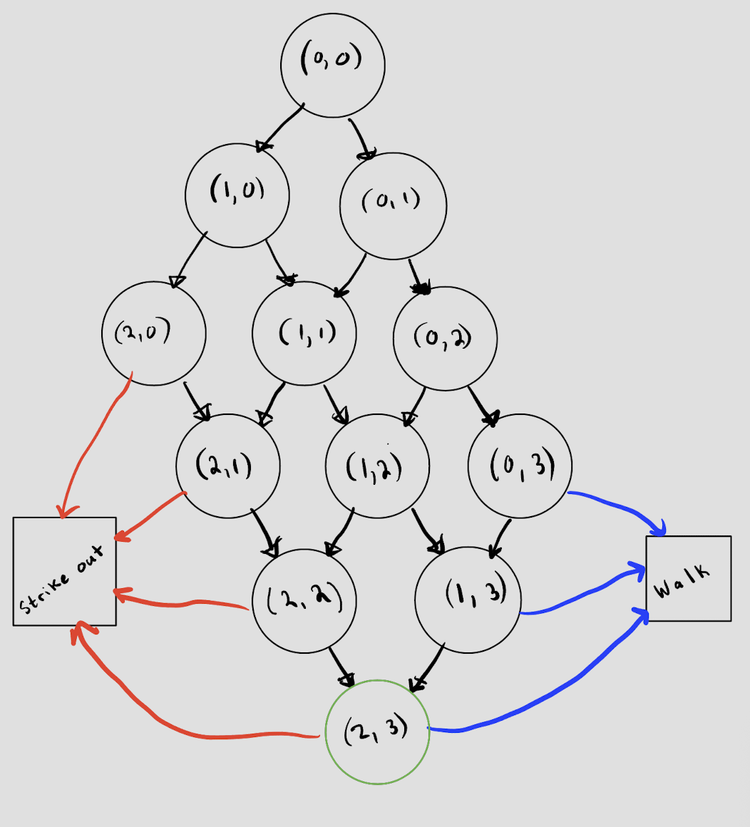
<p>We will have the absorption states: $(b, 3)$ and $(4, s)$ for $b \in[3]$ and $s \in [2]$ which represent the outcomes of <code class="language-plaintext highlighter-rouge">strikeout</code> and <code class="language-plaintext highlighter-rouge">walk</code> respectively, and an auxiliary state that represents a <code class="language-plaintext highlighter-rouge">Homerun</code>, which can be reached from any non-terminal state in the game. We visualize the Markov chain below in Figure 1 (omitting the <code class="language-plaintext highlighter-rouge">Homerun</code> state for clarity).</p>

<figure>
    <img src="/assets/img/blog_images/2025-11-01-robot-baseball/MC.png" width="70%" style="display: block; margin: auto;" />
    <figcaption style="text-align: center;">Figure 1: Plot of the states of the Markov chain and their possible transitions. The Homerun state has been omitted but every state has the probability to end the game in a Homerun. The full-count state has been highlighted in <span style="color:green">green</span>. </figcaption>
</figure>

<p>Given that we are at the non-absorbing state $(b, s)$, we can either transition to $(b + 1, s)$, $(b, s + 1)$ or the <code class="language-plaintext highlighter-rouge">Homerun</code> state. Let $Q(b, s)$ be the probability of reaching a full count given we are at state $(b, s)$. We can write $Q(b,s)$ as</p>

\[Q(b, s) = {x}^2 \bigg(p \cdot 0 + (1-p) Q(b, s + 1)\bigg) + 2x(1-x) Q(b, s + 1) + (1 - x)^2 Q(b + 1, s)\]

<p>where $x$ is the Nash-equilibrium strategy given in (\ref{eq:y_strat}).  The base cases for our function $Q$ are  $Q(3, 2) = 1$ and $Q(b, s) = 0$ for any terminal state. For a given $p$, we can now use dynamic programming to compute $Q(0, 0)$, using the snippet of Mathematica code below. We want to know the value of $p \in [0,1]$ that maximizes the value of $Q(0, 0)$.</p>

<div class="language-mathematica highlighter-rouge"><div class="highlight"><pre class="highlight"><code><span class="c">(* Base Cases *)</span><span class="w">
</span><span class="nv">Q</span><span class="p">[</span><span class="nv">b</span><span class="o">_</span><span class="w"> </span><span class="o">/;</span><span class="w"> </span><span class="nv">b</span><span class="w"> </span><span class="o">==</span><span class="w"> </span><span class="nv">B</span><span class="w"> </span><span class="o">-</span><span class="w"> </span><span class="m">1</span><span class="o">,</span><span class="w"> </span><span class="nv">s</span><span class="o">_</span><span class="w"> </span><span class="o">/;</span><span class="w"> </span><span class="nv">s</span><span class="w"> </span><span class="o">==</span><span class="w"> </span><span class="nv">S</span><span class="w"> </span><span class="o">-</span><span class="w"> </span><span class="m">1</span><span class="p">]</span><span class="w"> </span><span class="o">:=</span><span class="w"> </span><span class="m">1</span><span class="w"> 
</span><span class="nv">Q</span><span class="p">[</span><span class="nv">b</span><span class="o">_</span><span class="w"> </span><span class="o">/;</span><span class="w"> </span><span class="nv">b</span><span class="w"> </span><span class="o">==</span><span class="w"> </span><span class="nv">B</span><span class="o">,</span><span class="w"> </span><span class="nv">s</span><span class="o">_</span><span class="p">]</span><span class="w"> </span><span class="o">:=</span><span class="w"> </span><span class="m">0</span><span class="w">
</span><span class="nv">Q</span><span class="p">[</span><span class="nv">b</span><span class="o">_,</span><span class="w"> </span><span class="nv">s</span><span class="o">_</span><span class="w"> </span><span class="o">/;</span><span class="w"> </span><span class="nv">s</span><span class="w"> </span><span class="o">==</span><span class="w"> </span><span class="nv">S</span><span class="w"> </span><span class="p">]</span><span class="w"> </span><span class="o">:=</span><span class="w"> </span><span class="m">0</span><span class="w">

</span><span class="c">(*General recurrence *)</span><span class="w">
</span><span class="nv">Q</span><span class="p">[</span><span class="nv">b</span><span class="o">_,</span><span class="w"> </span><span class="nv">s</span><span class="o">_</span><span class="p">]</span><span class="w"> </span><span class="o">:=</span><span class="w"> </span><span class="nv">Q</span><span class="p">[</span><span class="nv">b</span><span class="o">,</span><span class="w"> </span><span class="nv">s</span><span class="p">]</span><span class="w"> </span><span class="o">=</span><span class="w"> </span><span class="nv">x</span><span class="p">[</span><span class="nv">b</span><span class="o">,</span><span class="w"> </span><span class="nv">s</span><span class="p">]</span><span class="o">^</span><span class="m">2</span><span class="w"> </span><span class="p">(</span><span class="m">1</span><span class="w"> </span><span class="o">-</span><span class="w"> </span><span class="nv">p</span><span class="p">)</span><span class="w"> </span><span class="nv">Q</span><span class="p">[</span><span class="nv">b</span><span class="o">,</span><span class="w"> </span><span class="nv">s</span><span class="w"> </span><span class="o">+</span><span class="w"> </span><span class="m">1</span><span class="p">]</span><span class="w"> </span><span class="o">+</span><span class="w"> 
   </span><span class="m">2</span><span class="w"> </span><span class="nv">x</span><span class="p">[</span><span class="nv">b</span><span class="o">,</span><span class="w"> </span><span class="nv">s</span><span class="p">]</span><span class="w"> </span><span class="p">(</span><span class="m">1</span><span class="w"> </span><span class="o">-</span><span class="w"> </span><span class="nv">x</span><span class="p">[</span><span class="nv">b</span><span class="o">,</span><span class="w"> </span><span class="nv">s</span><span class="p">])</span><span class="w"> </span><span class="nv">Q</span><span class="p">[</span><span class="nv">b</span><span class="o">,</span><span class="w"> </span><span class="nv">s</span><span class="w"> </span><span class="o">+</span><span class="w"> </span><span class="m">1</span><span class="p">]</span><span class="w"> </span><span class="o">+</span><span class="w"> </span><span class="p">(</span><span class="m">1</span><span class="w"> </span><span class="o">-</span><span class="w"> </span><span class="nv">x</span><span class="p">[</span><span class="nv">b</span><span class="o">,</span><span class="w"> </span><span class="nv">s</span><span class="p">])</span><span class="w"> </span><span class="o">^</span><span class="m">2</span><span class="w"> </span><span class="nv">Q</span><span class="p">[</span><span class="nv">b</span><span class="w"> </span><span class="o">+</span><span class="w"> </span><span class="m">1</span><span class="o">,</span><span class="w"> </span><span class="nv">s</span><span class="p">]</span><span class="w">
</span></code></pre></div></div>

<h3 id="optimizing-for-a-full-count">Optimizing for a Full-Count.</h3>

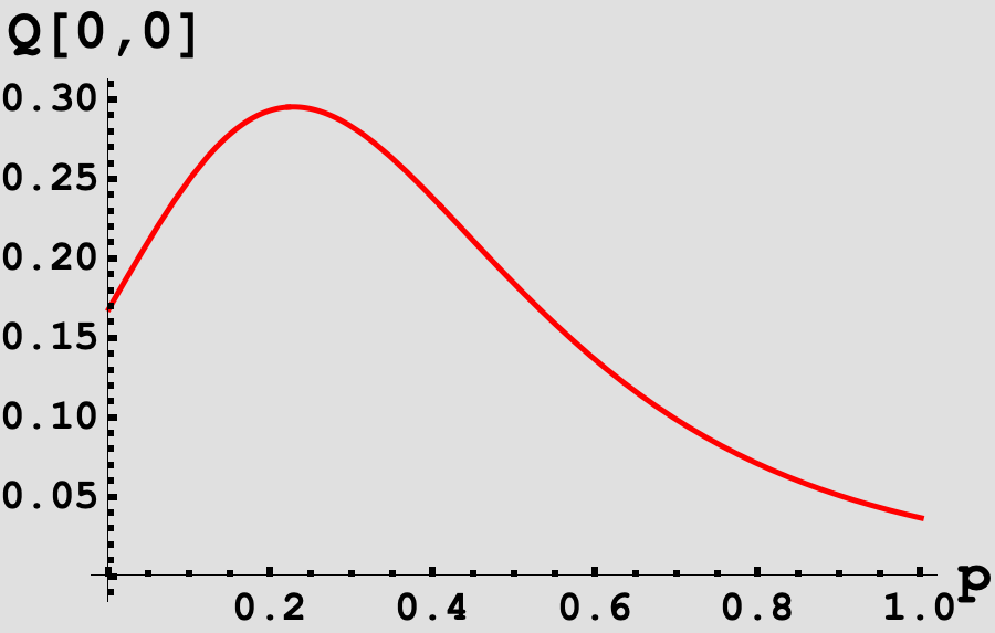
<p>We can plot $Q(0,0)$ as a function of $p$.</p>

<figure>
    <img src="/assets/img/blog_images/2025_08_01-robot-roadtrip/image.png" width="70%" style="display: block; margin: auto;" />
     <figcaption style="text-align: center;">Figure 2: The probability of reaching a full-count as a function of Homerun probability $p$.</figcaption>
</figure>

<p>Based on the figure, we can see the probability is unimodal in $p$ and we can use our favorite <code class="language-plaintext highlighter-rouge">Binary Search</code> method to determine the $p$ that maximizes our function. Alternatively, we can ask Mathematica to do this for us!</p>

<div class="language-mathematica highlighter-rouge"><div class="highlight"><pre class="highlight"><code><span class="c">(* Maximize Q[0,0] over the interval [0,1] *)</span><span class="w">
</span><span class="nb">NMaximize</span><span class="p">[{</span><span class="nv">Q</span><span class="p">[</span><span class="m">0</span><span class="o">,</span><span class="w"> </span><span class="m">0</span><span class="p">]</span><span class="o">,</span><span class="w"> </span><span class="nv">p</span><span class="w"> </span><span class="o">&gt;=</span><span class="w"> </span><span class="m">0</span><span class="o">,</span><span class="w"> </span><span class="nv">p</span><span class="w"> </span><span class="o">&lt;=</span><span class="w"> </span><span class="m">1</span><span class="p">}</span><span class="o">,</span><span class="w"> </span><span class="nv">p</span><span class="o">,</span><span class="w"> </span><span class="nb">WorkingPrecision</span><span class="w"> </span><span class="o">-&gt;</span><span class="w"> </span><span class="m">20</span><span class="p">]</span><span class="w">
</span></code></pre></div></div>

<p>Which produces a value of $\boxed{p^* \approx 0.2269732325}$ and the probability of reaching a full count in this case $\boxed{q \approx 0.2959679934}$, which is the answer to this month’s puzzle!</p>

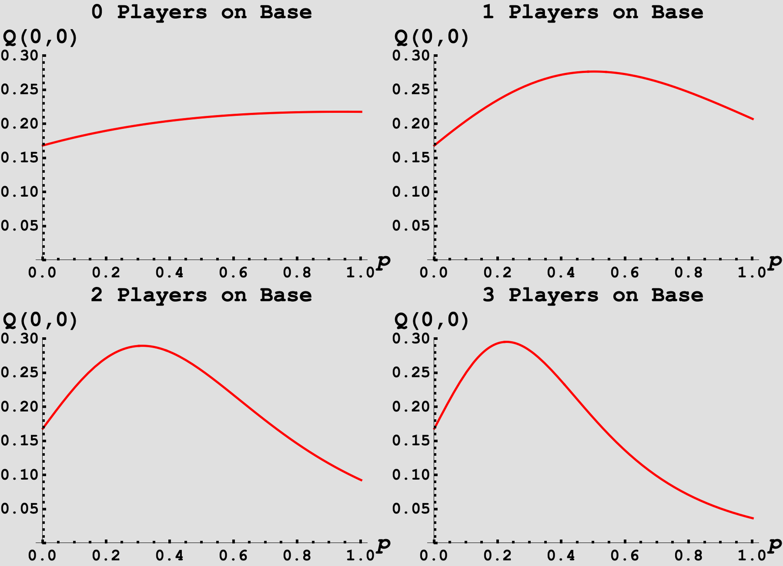
<p>For fun, I experimented with changing the value of the <code class="language-plaintext highlighter-rouge">Homerun</code> state. In the given description, the value of a <code class="language-plaintext highlighter-rouge">Homerun</code> is 4 which implies the Batter has the bases loaded! What if this was instead a lower stakes scenario for the pitcher, and there were instead fewer points on the line if the Batter hit a <code class="language-plaintext highlighter-rouge">Homerun</code>. Below are the probabilities of reaching a full count, for various numbers of runners on base, as a function of $p$. We can see that with more players on base, the lower the value of $p$ needs to be to maximize the odds of reaching a full count!</p>

<figure>
  <center>
  <img src="/assets/img/blog_images/2025-11-01-robot-baseball/q_evolution.gif" width="60%" style="display: block; margin: auto;" />
     <figcaption style="text-align: center;"> Figure 3. The probability of reaching a full-count given different numbers of players on base. </figcaption>
    </center>
</figure>

<div class="footnotes" role="doc-endnotes">
  <ol>
    <li id="fn:1">
      <p>Can you prove it? <a href="#fnref:1" class="reversefootnote" role="doc-backlink">&#8617;</a></p>
    </li>
  </ol>
</div>]]></content><author><name></name></author><category term="math," /><category term="programming" /><summary type="html"><![CDATA[My solution to the 2025 October Puzzle]]></summary></entry><entry><title type="html">Jane Street Puzzle: Robot Road Trip</title><link href="https://ccolombe12.github.io/blog/2025/robot-road-trip/" rel="alternate" type="text/html" title="Jane Street Puzzle: Robot Road Trip" /><published>2025-08-01T00:00:01+00:00</published><updated>2025-08-01T00:00:01+00:00</updated><id>https://ccolombe12.github.io/blog/2025/robot-road-trip</id><content type="html" xml:base="https://ccolombe12.github.io/blog/2025/robot-road-trip/"><![CDATA[<h2 id="problem-statement">Problem Statement</h2>
<blockquote>
  <p>Robot cars have a top speed (which they prefer to maintain at all times while driving) that’s a real number randomly drawn uniformly between $1$ and \(2\) miles per minute. A two-lane highway for robot cars has a fast-lane (with minimum speed \(a\)) and a slow-lane (with maximum speed \(a\)). When a faster car overtakes a slower car in the same lane, the slower car is required to decelerate to either change lanes (if both cars start in the fast-lane) or stop on the shoulder (if both cars start in the slow-lane). Robot cars decelerate and accelerate at a constant rate of $1$ mile per minute per minute, timed so the faster, overtaking car doesn’t have to change speed at all, and passing happens instantaneously.</p>
</blockquote>

<blockquote>
  <p><strong>If cars rarely meet (so you never have to consider a car meeting more than one other car on its trip, see Mathematical clarification below), and you want to minimize the miles not driven due to passing, what should \(a\) be set to, in miles per minute? Give your answer to 10 decimal places.</strong></p>
</blockquote>

<blockquote>
  <p><em>Mathematical clarification:</em>  Say car trips arrive at a rate of $z &gt; 0$ car trip beginnings per mile per minute, uniformly across the infinite highway (cars enter and exit their trips at their preferred speed due to on/off ramps), and car trips have a constant length of \(N\) miles. Define \(f(z,N)\) to be the value of $a$ that minimizes the expected lost distance per car trip due to passing. Find:</p>
</blockquote>

\[a^* = \lim_{N \to \infty} \lim_{z \to 0^+} f(z,N)\]

<hr />
<h2 id="solution">Solution</h2>

<p>At a high-level, our solution will do the following:</p>

<ul>
  <li>For car $C$ entering the roadway at a given location, time, and speed, determine the necessary conditions for another car to overtake $C$ during $C$’s journey.</li>
  <li>Determine, for each overtake, the total miles not driven due to passing</li>
  <li>Combine these two to determine the expected miles not driven due to passing for a car traveling at speed $v$.</li>
  <li>Average over all $v$ and determine the optimal speed threshold $f(z, N)$ for the highway.</li>
  <li>Determine $a^* = \lim_{N \to \infty} \lim_{z \to 0^+} f(z,N)$</li>
</ul>

<p>Before diving into the analysis, we will point out an observation from the mathematical clarification. Suppose we have an infinitely long highway at which cars enter at rate $z$ starts/mile/minute. Based on this description, we can say that the number of cars that enter the highway on a strip of length $\Delta x$ during a duration of time $\Delta t$ is a <a href="https://en.wikipedia.org/wiki/Poisson_distribution">Poisson random variable</a> with mean/rate $\lambda = z \Delta x \Delta t$. An important property of Poisson random variables is that their sum is also a Poisson random variable in which their rates have been added. With this in mind, we begin our analysis.</p>

<p>Let us consider a car $C$ that enters the highway (WLOG) at $x = 0$ and $t = 0$ with speed $v \in [1, 2]$. This car will travel for $N / v$ minutes and exit the highway at its destination $x = N$. We would like to determine the distribution for the number of cars will catch up to and pass $C$. First some observations. For a car $C’$ to pass car $C$, it must meeting the following conditions:</p>

<ul>
  <li>Have speed $u &gt; v$ (It is moving faster than $C$).</li>
  <li>If it starts its trip at time $t = t_s$, $C’$ must be behind where $C$ is at $t = t_s$ (It must start behind $C$ to overtake it).</li>
  <li>Share the same position as $C$ at some time $t$ during the time interval at which both cars are driving.</li>
</ul>

<p>Using these, we would like to get a distribution for the number of cars that will pass $C$.
Let us start by fixing the speed of car $C’$, to be some $u$ such that $u &gt; v$. What are the conditions on the starting time and position of $C’$ that will allow it to pass $C$? Suppose $C’$ starts at position $x_s$ at time $t_s$ and the two cars intersect at time $t$. Based the previous conditions, we get the following inequalities:</p>

\[\begin{align}
&amp; t_s \leq t \leq t_s + N/u &amp;&amp; (\text{intersect while $C'$ exists})  \\
&amp; 0 \leq t \leq N/v &amp;&amp; (\text{intersect while $C$ exists}) \\
&amp; x_s + u(t - t_s) = v t &amp;&amp; (\text{Both at same location at time $t$}) \label{eq:same_x}.
\end{align}\]

<p>Using (\ref{eq:same_x}), we can solve for $t$ as $t = \frac{u t_s - x_s}{u - v}$ and plug this into the other inequalities to get a set of four inequalities in the $(x_s, t_s)$-space.</p>

\[\begin{align}
&amp; t_s \leq \frac{u t_s - x_s}{u - v} \leq t_s + N/u  \\
&amp; 0 \leq \frac{u t_s - x_s}{u - v} \leq N/v \\
\end{align}\]

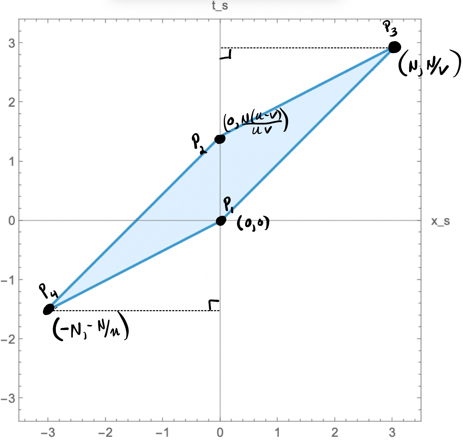
<p>Which when plotted in the $(x_s, t_s)$-space, these inequalities define a region $R$ which is a convex quadrilateral. This region is the set of all pairs of $(x_s, t_s)$ that would allow $C’$, traveling at speed $u$ to intersect $C$. See an example below.</p>

<figure>
    <img src="/assets/img/blog_images/2025_08_01-robot-roadtrip/fig1.png" width="70%" style="display: block; margin: auto;" />
     <figcaption style="text-align: center;">Figure 1: Example of the region in $(x_s, t_s)$-space, $R$, in which cars of speed $u$ will overtake $C$.</figcaption>
</figure>

<p>The vertices of $R$ are given by</p>

\[\begin{align*}
P_1 &amp; = (0, 0)\\
P_2 &amp; = (0, \frac{N(u - v)}{uv})\\
P_3 &amp; = (N, N/v) \\
P_4 &amp; = (-N, -N/u),
\end{align*}\]

<p>which imply that the area of our quadrilateral is \(\boxed{ Area(R) = \frac{N^2 (u - v)}{uv}}\).</p>

<p>Using our earlier observation about the number of cars for a given region of time and space being a Poisson random variable with parameter proportional to the area of that region, we deduce that the distribution for the number of  which cars of speed $u$ that arrive in the time-space region $R$ is a Poisson random variable with rate parameter $\lambda(u)$ given by</p>

\[\lambda(u) = z dF(u) \frac{N^2 (u - v)}{uv}  = z \frac{N^2 (u - v)}{uv} du.\]

<p>Where $z dF(u)$ is the rate at which car of speed $u$ arrive per mile per minute. Since the speed of cars is distributed $U(1, 2)$, we have $dF(u) = du / 1$.</p>

<p>We now have enough to compute the rate of overtakes for $C$ when it is in the slow-lane $\Lambda_S$ and when it is in the fast-lane, $\Lambda_F$.</p>

<p>For the slow-lane, we have</p>

\[\begin{align*}
\Lambda_S  &amp; = \int_v^a z \frac{N^2 (u - v)}{uv} du \\ 
&amp; = \frac{N^2 z \left(a  - v \log \left(\frac{a e}{v}\right)\right)}{v}.
\end{align*}\]

<p>And for the fast-lane</p>

\[\begin{align*}
\Lambda_F  &amp; = \int_v^2 \frac{N^2 (u - v)}{uv} du \\ 
&amp; = \frac{N^2 z \left(2  -v \log \left(\frac{2e}{v}\right)\right)}{v}.
\end{align*}\]

<p>These are the expected number of intersections per trip for a car of speed $v$, depending on whether the car is in the slow-lane or the fast-lane (since they are Poisson random variables). Now, we need to determine the “loss of distance traveled” for each overtake in either scenario.</p>

<p>Suppose we are in the slow-lane. Whenever we are passed, we must fully stop and then speed up to speed $v$ again. Since the acceleration is fixed to be $1$, the time it take to stop and speed up are the same and is $\delta t = v$ minutes. The total distance that would be traveled during this time without intersection is</p>

\[d_0 = v(\delta t + \delta t) = 2 v^2.\]

<p>On the other hand, when we have to stop, the distance traveled during the deceleration is</p>

\[d_1 = v \delta t - \frac{1}{2}(\delta t)^2 = v^2 / 2,\]

<p>and acceleration</p>

\[d_2 =\frac{1}{2}(\delta t)^2 = v^2 / 2.\]

<p>Thus the “loss of distance” for each passing in the slow-lane is:</p>

\[\begin{equation*}
\boxed{d_0 - d_1 - d_2 = v^2}. 
\end{equation*}\]

<p>By similar calculations, we find the “loss of distance” per passing in the fast-lane is:</p>

\[\boxed{(v - a)^2}.\]

<p>Putting these together, for a car of speed $v$ the expected lost distance due to passing, $\ell(v)$, is given by:</p>

\[\begin{align*}
\boxed{
\ell(v) = \begin{cases} v^2 \cdot \frac{N^2 z \left(a  - v \log \left(\frac{a e}{v}\right)\right)}{v} &amp; v \leq a \\
(v - a)^2  \cdot \frac{N^2 z \left(2  -v \log \left(\frac{2e}{v}\right)\right)}{v} &amp; v &gt; a
\end{cases}}
\end{align*}\]

<p>Since the speed of cars is distributed $U(1, 2)$, we need to compute the expected total lost distance for a car entering the highway with speed threshold $a$, denoted $L(a)$. We find</p>

\[\begin{align*}
L(a) &amp; = \int_{1}^2 \ell(v)\;  d v \\ 
     &amp; =\frac{1}{18} N^2 z \bigg(a^3 (18+\log (64))+18 a^2 (\log (4)-1)-6 \left(a^3+6 a^2-1\right) \log (a)-45 a+16\bigg).
\end{align*}\]

<p>Now, for fixed $z$ and $N$, we would like to find the value of $a$ that minimizes the above expression. However, note that $N$ and $z$ simply contribute a positive scaling factor and do not affect minimizing the overall expression. Therefore, it suffices to remove the constant factors and instead minimize the function</p>

\[g(a) := a^3 (18+\log (64))+18 a^2 (\log (4)-1)-6 \left(a^3+6 a^2-1\right) \log (a)-45 a+16.\]

<p>If we plot $g(a)$ over the interval $a \in [1,2]$, (see Figure 2) it appears that the function should have a unique minimizer over the desired interval.</p>

<figure>
    <img src="/assets/img/blog_images/2025_08_01-robot-roadtrip/fig2.pdf" width="70%" style="display: block; margin: auto;" />
    <figcaption style="text-align: center;">Figure 2: Plot of the loss function $g(a)$ over [1,2]</figcaption>
</figure>

<p>Unfortunately, there is not a nice closed form solution for the minimizer, so we will have to solve for it numerically. Doing so yields for fixed $N$ and $z$,</p>

\[\begin{equation*}
\boxed{f(z, N) = 1.177141417}
\end{equation*}\]

<p>taking the limit of which for $N$ and $z$ has no effect, and thus we have found the value of $a^*$ that minimizes the expected lost distance due to passing.</p>

<p>This value is pretty close to the minimum end of possible speeds on the highway! Around $82\%$ of the cars, on the highway are in the fast-lane. Why might that be? Well we can note that it is pretty expensive for a car in the slow-lane to be passed. Since $v \geq 1$ the loss of distance for every car in the slow-lane is at least $1$ whereas the maximum penalty for a passing in the fast-lane <em>is at most</em> 1. We see that passings in the slow-lane are much more expensive and thus we would need to have fewer of them than in the fast-lane in an optimal solution.</p>

<p>This was a fun problem that had me brushing up on my Poisson processes. I even found several problems in the Poisson Process section of <a href="https://www.amazon.com/Stochastic-Processes-Sheldon-M-Ross/dp/0471120626">Sheldon Ross’s Stochastic Processes textbook</a> that were about cars entering a highway according to a similar rule which served as a great warm-up to tackling this problem!</p>]]></content><author><name></name></author><category term="programming," /><category term="math" /><summary type="html"><![CDATA[My solution to the 2025 July Puzzle]]></summary></entry><entry><title type="html">Can You Throw the Hammer?</title><link href="https://ccolombe12.github.io/blog/2025/hammer_toss/" rel="alternate" type="text/html" title="Can You Throw the Hammer?" /><published>2025-04-21T00:00:00+00:00</published><updated>2025-04-21T00:00:00+00:00</updated><id>https://ccolombe12.github.io/blog/2025/hammer_toss</id><content type="html" xml:base="https://ccolombe12.github.io/blog/2025/hammer_toss/"><![CDATA[<p>This week’s <a href="https://thefiddler.substack.com">The Fiddler on the Proof</a> puzzle is paraphrased as follows:</p>

<blockquote>
  <p>You (Player 1) and your opponent (Player 2) are competing in a <a href="https://tglgolf.com">TGL golf match</a>. On any given hole you play, each of you has a 50-percent chance of winning the hole (and a zero percent chance of tying). That said, scorekeeping in this match is a little different from the norm.</p>
</blockquote>

<blockquote>
  <p>Each hole is worth 1 point. Before starting each hole, either you or your opponent can “throw the hammer.” When the hammer has been thrown, whoever did not throw the hammer must either accept the hammer or reject it. If they accept the hammer, the hole is worth 2 points. If they reject the hammer, they concede the hole and its 1 point to their opponent. Both players can throw the hammer on as many holes as they wish. (Should both players decide to throw the hammer at the exact same time—something that can’t be planned in advance—the hole is worth 2 points.)</p>
</blockquote>

<blockquote>
  <p>The first player to reach \(n\) points wins the match. Suppose all players always make rational decisions to maximize their own chances of winning. <strong>If the first player wins the first hole and the score is \((1 - 0)\) what is the probability that they win the match?</strong></p>
</blockquote>

<p><br /><br /></p>

<h2 id="solution"><strong>Solution</strong></h2>

<p>This is a quick one this week! For each round, the players are playing in a <a href="https://en.wikipedia.org/wiki/Zero-sum_game">zero-sum game</a>.We can view them as competing for the “resource” that is the probability that they win the overall game given the current round. To solve for the probability that Player 1 wins from the score-state \((1,0)\), which we denote as \(V(1, 0)\), we need to develop a recursive relationship for \(V(i, j)\), the probability that the first player wins from state \((i, j)\) (Player 1 has \(i\) points and Player 2 has \(j\) points).</p>

<p>We observe that, at the start of each turn each player has two actions to start the turn: throw the hammer or do not throw the hammer. In the case that they do not throw the hammer, then they may have to then make the secondary choice of “accept” or “reject” if the other player chooses to throw their hammer. We adopt the convention that Player 1 chooses their actions based on the objective of <em>maximizing</em> the probability that they win the overall game at state \((i, j)\), \(V(i, j)\). Conversely, Player 2 chooses actions with the objective of <em>minimizing</em> this \(V(i, j)\). This leads us to the recurrence relation:</p>

\[\begin{equation}
\begin{aligned}
V(i,j) = &amp;  \max\Bigl\{\,%
\underbrace{\min\bigl\{\tfrac12\,V(i+2,j) + \tfrac12\,V(i,j+2),\;V(i+1,j)\bigr\}}_{\text{Player 1 Tosses Hammer}},\\
&amp;\quad \underbrace{\min\Bigl\{\,
   \tfrac12\, V(i+1,j) + \tfrac12\,V(i,j+1),\;
   \max\bigl\{\tfrac12\,V(i+2,j) + \tfrac12\,V(i,j+2),\;V(i,j+1)\bigr\}
\Bigr\}}_{\text{Player 1 does not toss Hammer}} \Bigr\}. 
\end{aligned}\label{eq:rec}
\end{equation}\]

<p>With the base case(s) of</p>

\[\begin{align}
V(n, j)  = 1 &amp; \quad \forall \; j \in [n - 1] &amp;&amp; \text{(Player 1 has won)}\\
V(i, n)  = 0 &amp; \quad \forall \; i \in [n - 1] &amp;&amp; \text{(Player 1 has lost)}
\end{align}\]

<p>Here we can see Player 1 is taking the action that maximizes their probability of winning the game given that, if they took a particular action, Player 2 would choose the action to minimize Player 1’s probability of winning under that action. We see in (\ref{eq:rec}) that in the case Player 1 chooses not to hammer, they may then face a secondary decision to accept or reject a Player 2 hammer toss, in which they would again choose the probability-maximizing action.</p>

<p>We can code this recurrence up in python using <a href="https://www.geeksforgeeks.org/dynamic-programming/">Dynamic Programming</a> and visualize the probability of Player 1 winning at any given state. Here we have actually taken the liberty of slightly generalizing the problem. We are assuming that the Player 1’s probability of winning on round \(i + j\) (the current round, zero indexed) is known and is given by a list <code class="language-plaintext highlighter-rouge">hole_probs</code>. In the context of our original problem, every entry of <code class="language-plaintext highlighter-rouge">hole_probs</code> would be \(1/2\)</p>

<div class="language-python highlighter-rouge"><div class="highlight"><pre class="highlight"><code><span class="kn">from</span> <span class="n">functools</span> <span class="kn">import</span> <span class="n">cache</span>

<span class="nd">@cache</span>
<span class="k">def</span> <span class="nf">V</span><span class="p">(</span><span class="n">i</span><span class="p">,</span> <span class="n">j</span><span class="p">):</span>
    <span class="sh">"""</span><span class="s"> Probability Player 1 wins the game given we are at state (i, j) and they
    are playing to score n. We assume there is some list of probabilities 
    hole_probs such that hole_probs[i + j] is the probability that Player 1
    wins the current hole.  </span><span class="sh">"""</span>
    <span class="k">if</span> <span class="n">i</span> <span class="o">&gt;=</span> <span class="n">n</span><span class="p">:</span>
        <span class="k">return</span> <span class="mi">1</span>
    <span class="k">elif</span> <span class="n">j</span> <span class="o">&gt;=</span> <span class="n">n</span><span class="p">:</span>
        <span class="k">return</span> <span class="mi">0</span>

    <span class="c1"># the prob Player 1 wins current hole   
</span>    <span class="n">p</span> <span class="o">=</span> <span class="n">hole_probs</span><span class="p">[</span><span class="n">i</span> <span class="o">+</span> <span class="n">j</span><span class="p">]</span> 

    <span class="c1"># Player 1 hammers
</span>    <span class="n">prob_toss_win</span> <span class="o">=</span> <span class="nf">min</span><span class="p">(</span>
        <span class="n">p</span> <span class="o">*</span> <span class="nc">V</span><span class="p">(</span><span class="n">i</span> <span class="o">+</span> <span class="mi">2</span><span class="p">,</span> <span class="n">j</span><span class="p">)</span> <span class="o">+</span> <span class="p">(</span><span class="mi">1</span> <span class="o">-</span> <span class="n">p</span><span class="p">)</span> <span class="o">*</span> <span class="nc">V</span><span class="p">(</span><span class="n">i</span><span class="p">,</span> <span class="n">j</span> <span class="o">+</span> <span class="mi">2</span><span class="p">),</span> 
        <span class="nc">V</span><span class="p">(</span><span class="n">i</span> <span class="o">+</span> <span class="mi">1</span><span class="p">,</span> <span class="n">j</span><span class="p">)</span>
        <span class="p">)</span>

    <span class="c1"># Player 1 does not hammer
</span>    <span class="n">prob_pass_win</span> <span class="o">=</span> <span class="nf">min</span><span class="p">(</span>
        <span class="n">p</span> <span class="o">*</span> <span class="nc">V</span><span class="p">(</span><span class="n">i</span> <span class="o">+</span> <span class="mi">1</span><span class="p">,</span> <span class="n">j</span><span class="p">)</span> <span class="o">+</span> <span class="p">(</span><span class="mi">1</span> <span class="o">-</span> <span class="n">p</span><span class="p">)</span> <span class="o">*</span> <span class="nc">V</span><span class="p">(</span><span class="n">i</span><span class="p">,</span> <span class="n">j</span> <span class="o">+</span> <span class="mi">1</span><span class="p">),</span>
        <span class="nf">max</span><span class="p">(</span>
            <span class="n">p</span> <span class="o">*</span> <span class="nc">V</span><span class="p">(</span><span class="n">i</span> <span class="o">+</span> <span class="mi">2</span><span class="p">,</span> <span class="n">j</span><span class="p">)</span> <span class="o">+</span> <span class="p">(</span><span class="mi">1</span> <span class="o">-</span> <span class="n">p</span><span class="p">)</span> <span class="o">*</span> <span class="nc">V</span><span class="p">(</span><span class="n">i</span><span class="p">,</span> <span class="n">j</span> <span class="o">+</span> <span class="mi">2</span><span class="p">),</span>
            <span class="nc">V</span><span class="p">(</span><span class="n">i</span><span class="p">,</span> <span class="n">j</span> <span class="o">+</span> <span class="mi">1</span><span class="p">)</span>
            <span class="p">)</span>
     <span class="p">)</span>

    <span class="k">return</span> <span class="nf">max</span><span class="p">(</span><span class="n">prob_toss_win</span><span class="p">,</span> <span class="n">prob_pass_win</span><span class="p">)</span>  

<span class="c1"># now input problem specific parameters and solve 
</span><span class="n">n</span> <span class="o">=</span> <span class="mi">5</span>
<span class="n">hole_probs</span> <span class="o">=</span> <span class="p">[</span><span class="mi">1</span><span class="o">/</span><span class="mi">2</span> <span class="k">for</span> <span class="n">_</span> <span class="ow">in</span> <span class="nf">range</span><span class="p">(</span><span class="mi">2</span> <span class="o">*</span> <span class="n">n</span><span class="p">)]</span>
<span class="nf">print</span><span class="p">(</span><span class="sa">f</span><span class="sh">'</span><span class="s"> The probability of Player 1 winning is </span><span class="si">{</span><span class="nc">V</span><span class="p">(</span><span class="mi">1</span><span class="p">,</span><span class="mi">0</span><span class="p">)</span><span class="si">}</span><span class="sh">'</span><span class="p">)</span>
</code></pre></div></div>
<p>With this, we can get visualize the probability of Player 1 winning from any state. Here are two examples of the original problem (each player is equally skilled) for small and large \(n\).</p>
<figure style="max-width: 100%;">
  <div style="display: flex; justify-content: space-between; align-items: flex-start;">
    <div style="width: 48%;">
      <img src="/assets/img/blog_images/2025-04-18-hammer/winning_heatmap.png" style="width: 100%; display: block;" alt="Heatmap small" />
    </div>
    <div style="width: 48%;">
      <img src="/assets/img/blog_images/2025-04-18-hammer/heatmap_2_5050.png" style="width: 100%; display: block;" alt="Heatmap large" />
    </div>
  </div>
  <figcaption style="text-align: center; margin-top: 0.5em;">
    Comparison of win‑probability heatmaps (Player 1 perspective) for equally skilled opponents: \(n = 5\) on the left and \(n = 50\) on the right.
  </figcaption>
</figure>

<p>It’s worth noting that <strong>the “no hammer” option is never used by either player in this setting</strong>. For any \(n\) we can compute the value of \(V(1,0)\) in \(\mathcal{O}(n^2)\) time using our dynamic programming approach. For small \(n\), Player 1 has a significant advantage (for example \(n =3\) has \(V(1, 0) = 3/4\)) but as \(n\) increases, the value of \(V(1, 0)\) approaches \(1/2\) as we might expect.</p>

<p>Just for fun, we can also test out a different <code class="language-plaintext highlighter-rouge">hole_probs</code> distribution and see how this changes things. One interesting scenario is when Player 1 gradually improves over time. Specifically, at state \((i, j)\) the probability that they win the round is given by</p>

\[p_{ij} = \frac{i + j}{2n - 2}\]

<p>(as the round number increases Player 1 gets linearly better). Initially Player 1 would be very bad and unlikely to win, but in the higher rounds they would be increasingly more clutch over Player 2.</p>

<p>The win‑probability heatmaps now look like the figures below, revealing three asymmetric regions of the state space (one favoring each player and one where they are neutral). In this case, we see the “no hammer” option become used more widely.</p>
<figure style="max-width: 100%;">
  <div style="display: flex; justify-content: space-between; align-items: flex-start;">
    <div style="width: 48%;">
      <img src="/assets/img/blog_images/2025-04-18-hammer/heatmap_3_clutch.png" style="width: 100%; display: block;" alt="Heatmap small" />
    </div>
    <div style="width: 48%;">
      <img src="/assets/img/blog_images/2025-04-18-hammer/heatmap_clutch_larger.png" style="width: 100%; display: block;" alt="Heatmap large" />
    </div>
  </div>
  <figcaption style="text-align: center; margin-top: 0.5em;">
    Comparison of win‑probability heatmaps (Player 1 perspective) when Player 1 gets increasingly better (linearly): \(n = 50\) on the left and \(n = 300\) on the right.
  </figcaption>
</figure>

<p>Lastly, here is one more scenario where</p>

\[p_{ij} = \left(\frac{i + j}{2n - 2}\right)^2\]

<p>Here Player 1 still improves over the rounds but their skill grows quadratically. See if you can come up with your own funky distribution and see what the heatmap looks like using the code above and below!</p>

<figure style="max-width: 100%;">
  <div style="display: flex; justify-content: space-between; align-items: flex-start;">
    <div style="width: 48%;">
      <img src="/assets/img/blog_images/2025-04-18-hammer/heatmap_quad50.png" style="width: 100%; display: block;" alt="Heatmap small" />
    </div>
    <div style="width: 48%;">
      <img src="/assets/img/blog_images/2025-04-18-hammer/heatmap_quad_300.png" style="width: 100%; display: block;" alt="Heatmap large" />
    </div>
  </div>
  <figcaption style="text-align: center; margin-top: 0.5em;">
    Comparison of win‑probability heatmaps (Player 1 perspective) when Player 1 gets increasingly better (quadratic): \(n = 50\) on the left and \(n = 300\) on the right.
  </figcaption>
</figure>

<div class="language-python highlighter-rouge"><div class="highlight"><pre class="highlight"><code><span class="kn">import</span> <span class="n">matplotlib.pyplot</span> <span class="k">as</span> <span class="n">plt</span>
<span class="kn">import</span> <span class="n">numpy</span> <span class="k">as</span> <span class="n">np</span>
<span class="n">n</span> <span class="o">=</span> <span class="mi">5</span>
<span class="n">hole_probs</span> <span class="o">=</span> <span class="p">[</span><span class="mi">1</span><span class="o">/</span><span class="mi">2</span> <span class="k">for</span> <span class="n">_</span> <span class="ow">in</span> <span class="nf">range</span><span class="p">(</span><span class="mi">2</span> <span class="o">*</span> <span class="n">n</span> <span class="o">+</span> <span class="mi">1</span><span class="p">)]</span>
<span class="c1">#hole_probs = [i / (2 * n  - 2) for i in range(2 * n - 1)]
#hole_probs = [np.sqrt(i / (2 * n  - 2)) for i in range(2 * n - 1)]
#hole_probs = [(i / (2 * n  - 2)) ** 2 for i in range(2 * n - 1)]
</span><span class="nf">print</span><span class="p">(</span><span class="sa">f</span><span class="sh">'</span><span class="s">for n = </span><span class="si">{</span><span class="n">n</span><span class="si">}</span><span class="s">, the probability of Player 1 winning from the start is </span><span class="si">{</span><span class="nc">V</span><span class="p">(</span><span class="mi">0</span><span class="p">,</span> <span class="mi">0</span><span class="p">)</span><span class="si">:</span><span class="p">.</span><span class="mi">4</span><span class="n">f</span><span class="si">}</span><span class="s"> and with a 1 point lead is </span><span class="si">{</span><span class="nc">V</span><span class="p">(</span><span class="mi">1</span><span class="p">,</span> <span class="mi">0</span><span class="p">)</span><span class="si">:</span><span class="p">.</span><span class="mi">4</span><span class="n">f</span><span class="si">}</span><span class="sh">'</span><span class="p">)</span>
<span class="k">def</span> <span class="nf">plot_prob_win_heatmap</span><span class="p">(</span><span class="n">n</span><span class="p">):</span>
    <span class="sh">"""</span><span class="s"> heatmap of win probabilities V(i, j) for 0 &lt;= i, j &lt; n.</span><span class="sh">"""</span>
    <span class="c1"># matrix of V(i, j) 
</span>    <span class="n">M</span> <span class="o">=</span> <span class="n">np</span><span class="p">.</span><span class="nf">zeros</span><span class="p">((</span><span class="n">n</span> <span class="o">+</span> <span class="mi">1</span><span class="p">,</span> <span class="n">n</span> <span class="o">+</span> <span class="mi">1</span><span class="p">))</span>
    <span class="k">for</span> <span class="n">i</span> <span class="ow">in</span> <span class="nf">range</span><span class="p">(</span><span class="n">n</span> <span class="o">+</span> <span class="mi">1</span><span class="p">):</span>
        <span class="k">for</span> <span class="n">j</span> <span class="ow">in</span> <span class="nf">range</span><span class="p">(</span><span class="n">n</span> <span class="o">+</span> <span class="mi">1</span><span class="p">):</span>
            <span class="n">M</span><span class="p">[</span><span class="n">i</span><span class="p">,</span> <span class="n">j</span><span class="p">]</span> <span class="o">=</span> <span class="nf">float</span><span class="p">(</span><span class="nc">V</span><span class="p">(</span><span class="n">j</span><span class="p">,</span> <span class="n">i</span><span class="p">))</span>
    
    <span class="c1"># plot the heatmap
</span>    <span class="n">plt</span><span class="p">.</span><span class="nf">figure</span><span class="p">(</span><span class="n">figsize</span><span class="o">=</span><span class="p">(</span><span class="mi">8</span><span class="p">,</span> <span class="mi">6</span><span class="p">))</span>
    <span class="n">plt</span><span class="p">.</span><span class="nf">imshow</span><span class="p">(</span><span class="n">M</span><span class="p">,</span> <span class="n">origin</span><span class="o">=</span><span class="sh">'</span><span class="s">lower</span><span class="sh">'</span><span class="p">,</span> <span class="n">cmap</span><span class="o">=</span><span class="sh">'</span><span class="s">RdYlGn</span><span class="sh">'</span><span class="p">,</span> <span class="n">interpolation</span><span class="o">=</span><span class="sh">'</span><span class="s">nearest</span><span class="sh">'</span><span class="p">)</span>
    <span class="n">plt</span><span class="p">.</span><span class="nf">colorbar</span><span class="p">(</span><span class="n">label</span><span class="o">=</span><span class="sh">'</span><span class="s">Probability of Win</span><span class="sh">'</span><span class="p">)</span>
    <span class="n">plt</span><span class="p">.</span><span class="nf">xlabel</span><span class="p">(</span><span class="sa">r</span><span class="sh">'</span><span class="s">$i$, Player 1 score</span><span class="sh">'</span><span class="p">)</span>
    <span class="n">plt</span><span class="p">.</span><span class="nf">ylabel</span><span class="p">(</span><span class="sa">r</span><span class="sh">'</span><span class="s">$j$, Player 2 score</span><span class="sh">'</span><span class="p">)</span>
    <span class="n">plt</span><span class="p">.</span><span class="nf">title</span><span class="p">(</span><span class="sa">fr</span><span class="sh">'</span><span class="s">Player $1$ Win Probability Heatmap for $n = </span><span class="si">{</span><span class="n">n</span><span class="si">}</span><span class="s">$</span><span class="sh">'</span><span class="p">)</span>
    <span class="n">plt</span><span class="p">.</span><span class="nf">show</span><span class="p">()</span>

<span class="c1"># try it out 
</span><span class="nf">plot_prob_win_heatmap</span><span class="p">(</span><span class="n">n</span><span class="p">)</span>

</code></pre></div></div>]]></content><author><name></name></author><summary type="html"><![CDATA[My solution to this week's Fiddler on the Proof Puzzle]]></summary></entry><entry><title type="html">Can You Solve a High Schooler’s Favorite Puzzle?</title><link href="https://ccolombe12.github.io/blog/2025/HS_fav_puzzle/" rel="alternate" type="text/html" title="Can You Solve a High Schooler’s Favorite Puzzle?" /><published>2025-04-08T00:00:00+00:00</published><updated>2025-04-08T00:00:00+00:00</updated><id>https://ccolombe12.github.io/blog/2025/HS_fav_puzzle</id><content type="html" xml:base="https://ccolombe12.github.io/blog/2025/HS_fav_puzzle/"><![CDATA[<p>This week’s <a href="https://thefiddler.substack.com">The Fiddler on the Proof</a> puzzle is paraphrased as follows:</p>

<blockquote>
  <p>A teacher is handing out candy to his \(N\) students, of which \(N \geq 4\). He abides by the following rules:</p>
</blockquote>

<blockquote>
  <p>He hands out candy to groups of three students (i.e., “trios”) at a time. Each member of the trio gets one piece of candy. Each unique trio can ask for candy, but that same trio can’t come back for seconds. If students in the trio want more candy, they must return as part of a different trio.
When a trio gets candy, the next trio can’t contain any students from that previous trio.</p>
</blockquote>

<blockquote>
  <p>It turns out that <em>every</em> possible trio can get a helping of candy. <strong>What is the smallest class size \(N\) for which this is possible?</strong></p>
</blockquote>

<p><br /><br /></p>
<h2 id="solution">Solution</h2>

<p>Instead of focusing on the case of trios, we will generalize the problem and consider groups of \(k\) students. If there is some ordering of groups such that every group of \(k\) students can receive candy, what is the smallest such \(N\) for which this is possible? Denote this smallest \(N\) as \(N(k)\).</p>

<p>Now, what are some initial observations we can make about the problem? Well, first off, we can actually place the lower bound that \(N(k) \geq 2 k + 1\). This is because if there are any fewer students, then we cannot find a sequence of 3 initial \(k\)-groups. This was the only bound I could find in my initial exploration—the problem turned out to be much harder than I expected!</p>

<p>Perhaps changing our perspective can help us gain traction on the problem. What if we instead thought of the students as <strong>nodes</strong> in a graph and two nodes share an <strong>edge</strong> only if their representative groups are disjoint. Now, a <a href="https://en.wikipedia.org/wiki/Path_(graph_theory)">path</a> in this graph would then represent a sequence of groups that could get candy such that every group in the sequence is disjoint from the groups adjacent to it in the sequence. If we could find a path such that every node appeared in it exactly once, then we would have found a sequence of groups that allows every group to get candy! Such a path in a graph where every node is visited exactly once is called a <a href="https://en.wikipedia.org/wiki/Hamiltonian_path">Hamiltonian path</a>. Our problem has now become, for what \(N\) does a Hamiltonian path exist for a given \(k\)?</p>

<p>It turns out that determining whether a Hamiltonian path exists in a graph <em>is a <a href="https://en.wikipedia.org/wiki/NP-completeness">hard problem</a></em>. But perhaps there are some special properties our graph that make it a tractable endeavor without having to perform a brute-force search.</p>

<p>We need to first better describe our graph. Suppose for now, we fix some \(N \geq 2 k + 1\) and construct our graph as follows:
The set of nodes \(V\) is the set of subsets of size \(k\) from the group of \(N\) students. Nodes \(u, v \in V\) share an undirected edge if \(u \cap v = \emptyset\). This graph will have \(\binom{N}{k}\) nodes. For a given node \(u\), it will have \(\binom{N - k}{k}\) edges (one to each of the groups that it shares no members with) and thus by the handshake lemma, the graph has \(\frac{\binom{N}{k}\binom{N - k}{k}}{2}\) edges.</p>

<p>Now that we have a clearer picture of the graph, is there a particular aspect of it that allows us to determine if it has a Hamiltonian path? It turns out there is. One especially nice property of our graph is that it is <em>vertex transitive</em>. In simple terms, vertex transitive implies that from every node in the graph, the graph “looks the same” from the perspective of that node. It turns out that there is an open conjecture, the <a href="https://en.wikipedia.org/wiki/Lovász_conjecture">Lovász Conjecture</a> that states:</p>
<blockquote>
  <p><em>Lovász conjecture: Every finite, connected, vertex regular graph has a Hamiltonian cycle (and thus a Hamiltonian path).</em></p>
</blockquote>

<p>While this is an open conjecture, it implies that there is some evidence to suggest: as long as our choice of \(N\) allows our graph to be connected, since it is vertex transitive, it may indeed contain a Hamiltonian path. This leads us to the natural question, for what \(N\) is our graph connected?</p>

<p>It turns out that for \(N \geq 2k + 1\), our graph is connected! To see why, consider any two distinct nodes \(u, v \in V\). If \(u \cap v = \emptyset\), then they share an edge by definition. Otherwise, Suppose \(u\) represents the group of students \((A, S)\) and \(v\) represents the students \((B, S)\) where \(A \cap B = \emptyset\) and \(\|S\| = x\). Under this framing, we can show that that the set of students \(W\) that are not in  \(u \cup v\) has size \(x + 1\). We can now construct a path from \(u \to v\) using the following intuition.</p>

<p>We make a path that has the form</p>

\[(A, S) \to (B, W') \to (A, S') \to (B, W'') \to (A, S'')\to   \dots \to (B, S)\]

<p>where we use the extra student in \(W\) to iteratively swap in one more student of \(S\) into the group with \(B\) and vice versa until the subgroup paired with the \(B\) subgroup eventually becomes the desired \(S\) subgroup <sup id="fnref:1"><a href="#fn:1" class="footnote" rel="footnote" role="doc-noteref">1</a></sup>.</p>

<p>Now that we have argued that \(N=2k + 1\) is sufficient for our graph to be connected, and we have “evidence” now that suggests this should also be sufficient for there to exist a hamiltonian path, what else can we do except also conjecture that \(N(k) = 2k + 1\) and call it a day? Well it turns out that our graph with \(N = 2k + 1\) nodes is actually a special and well-studied graph. It turns out for \(N = 2 k + 1\), we have actually described the <em><a href="https://en.wikipedia.org/wiki/Odd_graph">Odd Graph</a></em>, \(O_{k + 1}\) which, for \(k \geq 3\),  <strong>is known to contain a Hamiltonian cycle (and thus a path)!</strong><sup id="fnref:2"><a href="#fn:2" class="footnote" rel="footnote" role="doc-noteref">2</a></sup>  Therefore, our choice of \(N = 2k + 1\) will ensure that every grouping of children can get candy and since this is the lower bound on possible values of \(N\), we indeed have that</p>

\[\boxed{N(k) = 2k + 1}.\]

<div class="footnotes" role="doc-endnotes">
  <ol>
    <li id="fn:1">
      <p>To really see how this works, try to do this with the case of \(k= 3\) and \(N = 7\). <a href="#fnref:1" class="reversefootnote" role="doc-backlink">&#8617;</a></p>
    </li>
    <li id="fn:2">
      <p>A bit anticlimactic that we’re able that we are able to simply point to the literature and call it a day but, but that’s research sometimes! This was a great problem to learn more graph theory! <a href="#fnref:2" class="reversefootnote" role="doc-backlink">&#8617;</a></p>
    </li>
  </ol>
</div>]]></content><author><name></name></author><summary type="html"><![CDATA[My solution to this week's Fiddler on the Proof Puzzle]]></summary></entry><entry><title type="html">Can You Grow a Hibiscus Hedge?</title><link href="https://ccolombe12.github.io/blog/2025/hibiscus-hedge/" rel="alternate" type="text/html" title="Can You Grow a Hibiscus Hedge?" /><published>2025-04-08T00:00:00+00:00</published><updated>2025-04-08T00:00:00+00:00</updated><id>https://ccolombe12.github.io/blog/2025/hibiscus-hedge</id><content type="html" xml:base="https://ccolombe12.github.io/blog/2025/hibiscus-hedge/"><![CDATA[<p>This week’s <a href="https://thefiddler.substack.com">The Fiddler on the Proof</a> puzzle is paraphrased as follows:</p>

<blockquote>
  <p><strong>Part 1:</strong>  You have many flowers in three colors: red, orange, and yellow. You want to plant them in a straight row such that the order appears somewhat random, but not truly random. More specifically, you want the following to be true:</p>
  <ul>
    <li>No two adjacent flowers have the same color.</li>
    <li>No ordering of three consecutive flowers appears more than once in the row.</li>
  </ul>
</blockquote>

<blockquote>
  <p><strong>What is the maximum number of flowers the row can contain?</strong></p>
</blockquote>

<blockquote>
  <p><strong>Part 2:</strong>  In addition to red, orange, and yellow flowers, you now have a fourth color: pink! Again, you want to plant a straight row of flowers that appears somewhat random. The new rules are:</p>
  <ul>
    <li>No two adjacent flowers have the same color.</li>
    <li>No ordering of four consecutive flowers appears more than once in the flower row.</li>
    <li>Among any group of four consecutive flowers, at least three distinct colors are represented.</li>
  </ul>
</blockquote>

<blockquote>
  <p><strong>What is the maximum number of flowers the row can contain now?</strong></p>
</blockquote>

<p><br /><br /></p>

<h2 id="solution"><strong>Solution</strong></h2>

<h3 id="part-1"><strong>Part 1:</strong></h3>

<p>Let’s first establish an upper bound on how long our row of flowers <em>could</em> be. Since each possible pattern of three flowers can appear only once, the longest imaginable row contains each pattern exactly once. The total number of patterns can be calculated:</p>
<ul>
  <li>\(3\) choices for the first color</li>
  <li>\(2\) for the second</li>
  <li>\(2\) for the final color</li>
</ul>

<p>Which gives the grand total of \(12\) total color patterns. As each pattern overlaps by two flowers, the longest possible row length is \(14\). But, can we achieve this maximum?</p>

<p>We verify using backtracking with Python</p>

<div class="language-python highlighter-rouge"><div class="highlight"><pre class="highlight"><code><span class="kn">from</span> <span class="n">matplotlib.patches</span> <span class="kn">import</span> <span class="n">Rectangle</span>
<span class="c1"># lets write a function that, given the current state, sees how many flowers we can place
</span><span class="n">colors</span> <span class="o">=</span> <span class="p">[</span><span class="sh">'</span><span class="s">r</span><span class="sh">'</span><span class="p">,</span> <span class="sh">'</span><span class="s">o</span><span class="sh">'</span><span class="p">,</span> <span class="sh">'</span><span class="s">y</span><span class="sh">'</span><span class="p">]</span>

<span class="c1"># we need to write some helpers that allow us to check if we can place a color 
# given the current sequence of colors so far 
</span>
<span class="c1"># check the triplet formed is not a repeat 
</span><span class="k">def</span> <span class="nf">no_triplet</span><span class="p">(</span><span class="n">state</span><span class="p">,</span> <span class="n">color</span><span class="p">):</span>
    <span class="k">if</span> <span class="nf">len</span><span class="p">(</span><span class="n">state</span><span class="p">)</span> <span class="o">&lt;</span> <span class="mi">3</span><span class="p">:</span>
        <span class="k">return</span> <span class="bp">True</span>
    <span class="k">else</span><span class="p">:</span>
        <span class="n">cur_triplet</span> <span class="o">=</span> <span class="n">state</span><span class="p">[</span><span class="o">-</span><span class="mi">2</span><span class="p">:]</span> <span class="o">+</span> <span class="n">color</span>
        <span class="k">for</span> <span class="n">i</span> <span class="ow">in</span> <span class="nf">range</span><span class="p">(</span><span class="nf">len</span><span class="p">(</span><span class="n">state</span><span class="p">)</span> <span class="o">-</span> <span class="mi">2</span><span class="p">):</span>
            <span class="k">if</span> <span class="n">state</span><span class="p">[</span><span class="n">i</span><span class="p">:</span><span class="n">i</span><span class="o">+</span><span class="mi">3</span><span class="p">]</span> <span class="o">==</span> <span class="n">cur_triplet</span><span class="p">:</span>
                <span class="k">return</span> <span class="bp">False</span>
        <span class="k">return</span> <span class="bp">True</span>

<span class="c1"># check for adjacent color and not a new triplet 
</span><span class="k">def</span> <span class="nf">can_place</span><span class="p">(</span><span class="n">state</span><span class="p">,</span> <span class="n">color</span><span class="p">):</span>
    <span class="k">if</span> <span class="n">state</span><span class="p">[</span><span class="o">-</span><span class="mi">1</span><span class="p">]</span> <span class="o">!=</span> <span class="n">color</span> <span class="ow">and</span> <span class="nf">no_triplet</span><span class="p">(</span><span class="n">state</span><span class="p">,</span> <span class="n">color</span><span class="p">):</span>
        <span class="k">return</span> <span class="bp">True</span>
    <span class="k">return</span> <span class="bp">False</span>

<span class="c1"># returns the max len flower array given the current placement
</span><span class="k">def</span> <span class="nf">max_flower</span><span class="p">(</span><span class="n">state</span><span class="p">):</span>
    <span class="n">best</span> <span class="o">=</span> <span class="nf">len</span><span class="p">(</span><span class="n">state</span><span class="p">)</span>
    <span class="n">best_flower</span> <span class="o">=</span> <span class="n">state</span>
    <span class="k">for</span> <span class="n">color</span> <span class="ow">in</span> <span class="n">colors</span><span class="p">:</span>
        <span class="k">if</span> <span class="nf">can_place</span><span class="p">(</span><span class="n">state</span><span class="p">,</span> <span class="n">color</span><span class="p">):</span>
            <span class="n">cur_flower</span><span class="p">,</span> <span class="n">cur_size</span> <span class="o">=</span> <span class="nf">max_flower</span><span class="p">(</span><span class="n">state</span> <span class="o">+</span> <span class="n">color</span><span class="p">)</span>
            <span class="k">if</span> <span class="n">cur_size</span> <span class="o">&gt;</span> <span class="n">best</span><span class="p">:</span>
                <span class="n">best</span> <span class="o">=</span> <span class="n">cur_size</span>
                <span class="n">best_flower</span> <span class="o">=</span> <span class="n">cur_flower</span>
    
    <span class="k">return</span> <span class="n">best_flower</span><span class="p">,</span> <span class="n">best</span>

<span class="c1"># just assume the base flower is 'ro'
</span><span class="n">best_flower</span><span class="p">,</span> <span class="n">best_size</span> <span class="o">=</span> <span class="nf">max_flower</span><span class="p">(</span><span class="sh">'</span><span class="s">ro</span><span class="sh">'</span><span class="p">)</span>
<span class="nf">print</span><span class="p">(</span><span class="sh">'</span><span class="s">Best flower:</span><span class="sh">'</span><span class="p">,</span> <span class="n">best_flower</span><span class="p">)</span>
<span class="nf">print</span><span class="p">(</span><span class="sh">'</span><span class="s">Best size:</span><span class="sh">'</span><span class="p">,</span> <span class="n">best_size</span><span class="p">)</span>


<span class="c1"># Now lets visualize the best flower as a sequence of rectangles 
</span><span class="kn">import</span> <span class="n">matplotlib.pyplot</span> <span class="k">as</span> <span class="n">plt</span>

<span class="n">color_mapping</span> <span class="o">=</span> <span class="p">{</span><span class="sh">'</span><span class="s">r</span><span class="sh">'</span><span class="p">:</span> <span class="sh">'</span><span class="s">red</span><span class="sh">'</span><span class="p">,</span> <span class="sh">'</span><span class="s">o</span><span class="sh">'</span><span class="p">:</span> <span class="sh">'</span><span class="s">orange</span><span class="sh">'</span><span class="p">,</span> <span class="sh">'</span><span class="s">y</span><span class="sh">'</span><span class="p">:</span> <span class="sh">'</span><span class="s">yellow</span><span class="sh">'</span><span class="p">}</span>

<span class="n">fig</span><span class="p">,</span> <span class="n">ax</span> <span class="o">=</span> <span class="n">plt</span><span class="p">.</span><span class="nf">subplots</span><span class="p">(</span><span class="n">figsize</span><span class="o">=</span><span class="p">(</span><span class="nf">len</span><span class="p">(</span><span class="n">best_flower</span><span class="p">),</span> <span class="mi">2</span><span class="p">))</span>
<span class="k">for</span> <span class="n">idx</span><span class="p">,</span> <span class="n">letter</span> <span class="ow">in</span> <span class="nf">enumerate</span><span class="p">(</span><span class="n">best_flower</span><span class="p">):</span>
    <span class="n">rect</span> <span class="o">=</span> <span class="nc">Rectangle</span><span class="p">((</span><span class="n">idx</span><span class="p">,</span> <span class="mi">0</span><span class="p">),</span> <span class="mi">1</span><span class="p">,</span> <span class="mi">1</span><span class="p">,</span> <span class="n">color</span><span class="o">=</span><span class="n">color_mapping</span><span class="p">[</span><span class="n">letter</span><span class="p">])</span>
    <span class="n">ax</span><span class="p">.</span><span class="nf">add_patch</span><span class="p">(</span><span class="n">rect</span><span class="p">)</span>
    
<span class="n">ax</span><span class="p">.</span><span class="nf">set_xlim</span><span class="p">(</span><span class="mi">0</span><span class="p">,</span> <span class="nf">len</span><span class="p">(</span><span class="n">best_flower</span><span class="p">))</span>
<span class="n">ax</span><span class="p">.</span><span class="nf">set_ylim</span><span class="p">(</span><span class="mi">0</span><span class="p">,</span> <span class="mi">1</span><span class="p">)</span>
<span class="n">ax</span><span class="p">.</span><span class="nf">axis</span><span class="p">(</span><span class="sh">'</span><span class="s">off</span><span class="sh">'</span><span class="p">)</span>
<span class="n">plt</span><span class="p">.</span><span class="nf">show</span><span class="p">()</span>
            
</code></pre></div></div>
<p>Which gives us the output and visualized longest flower:</p>
<div class="language-plaintext highlighter-rouge"><div class="highlight"><pre class="highlight"><code>Best flower: roroyryoyoryro
Best size: 14
</code></pre></div></div>

<figure>
  <center>
  <img src="/assets/img/blog_images/2025-04-11-hibiscus/bush.png" width="80%" style="display: block; margin: auto;" />
  <figcaption> An example of an optimal flower row of length 14 
</figcaption> 
</center>
</figure>

<p>Confirming that we can indeed reach the longest possible flower length of \(\boxed{14}\) under the conditions!</p>

<h2 id="part-2"><strong>Part 2</strong></h2>

<p>For the extra credit, we can still use the backtracking approach but given the increased state space size, it might take a while. We can try another approach to handle the larger state space <em>integer programming</em> with the <a href="https://www.microsoft.com/en-us/research/project/z3-3/">z3 module</a>. With this approach, we will answer the <a href="https://en.wikipedia.org/wiki/Decision_problem">decision problem</a>:</p>

<blockquote>
  <p>for a given \(n\), does there exist a feasible flower row of length \(n\)?</p>
</blockquote>

<p>Using the answer to this decision problem, we can <em>binary search</em> over the space of the possible lengths to find the largest \(n\) such that there exists a feasible flower row.</p>

<p>Before we implement this, we need to again place an upper bound on the largest possible flower row so that we know the range of sizes we are to search over. Using a similar logic as in Part 1, along with the additional constraint that for any \(4\) adjacent flowers we need at least \(3\) distinct colors, we can show that there are \(96\) such possible color patterns. Therefore the largest possible flower row has size \(99\). Now it remains to model the decision procedure with the z3 module in python and then binary search over the space of possible lengths \([4, 96]\).</p>

<div class="language-python highlighter-rouge"><div class="highlight"><pre class="highlight"><code><span class="kn">from</span> <span class="n">z3</span> <span class="kn">import</span> <span class="o">*</span>
<span class="kn">from</span> <span class="n">itertools</span> <span class="kn">import</span> <span class="n">combinations</span>

<span class="k">def</span> <span class="nf">flower_problem</span><span class="p">(</span><span class="n">n</span><span class="p">,</span> <span class="n">k</span><span class="o">=</span><span class="mi">4</span><span class="p">):</span>
    <span class="sh">"""</span><span class="s">The decision procedure: returns True if there exists a feasible flower row
    of size n with k colors. </span><span class="sh">"""</span>
    <span class="c1"># The n decision variables (color of each flower)
</span>    <span class="n">x</span> <span class="o">=</span> <span class="p">[</span><span class="nc">Int</span><span class="p">(</span><span class="sa">f</span><span class="sh">'</span><span class="s">x_</span><span class="si">{</span><span class="n">i</span><span class="si">}</span><span class="sh">'</span><span class="p">)</span> <span class="k">for</span> <span class="n">i</span> <span class="ow">in</span> <span class="nf">range</span><span class="p">(</span><span class="n">n</span><span class="p">)]</span>
    
    <span class="c1"># Constraints:
</span>    <span class="n">s</span> <span class="o">=</span> <span class="nc">Solver</span><span class="p">()</span>
    <span class="c1"># 1)  Each flower must have a color 
</span>    <span class="k">for</span> <span class="n">i</span> <span class="ow">in</span> <span class="nf">range</span><span class="p">(</span><span class="n">n</span><span class="p">):</span>
        <span class="n">s</span><span class="p">.</span><span class="nf">add</span><span class="p">(</span><span class="nc">And</span><span class="p">(</span><span class="n">x</span><span class="p">[</span><span class="n">i</span><span class="p">]</span> <span class="o">&gt;=</span> <span class="mi">0</span><span class="p">,</span> <span class="n">x</span><span class="p">[</span><span class="n">i</span><span class="p">]</span> <span class="o">&lt;=</span> <span class="n">k</span> <span class="o">-</span> <span class="mi">1</span><span class="p">))</span>
    
    <span class="c1"># 2) No two adjacent colors match
</span>    <span class="k">for</span> <span class="n">i</span> <span class="ow">in</span> <span class="nf">range</span><span class="p">(</span><span class="n">n</span> <span class="o">-</span> <span class="mi">1</span><span class="p">):</span>
        <span class="n">s</span><span class="p">.</span><span class="nf">add</span><span class="p">(</span><span class="n">x</span><span class="p">[</span><span class="n">i</span><span class="p">]</span> <span class="o">!=</span> <span class="n">x</span><span class="p">[</span><span class="n">i</span><span class="o">+</span><span class="mi">1</span><span class="p">])</span>
    
    <span class="c1"># 3) no repeated k-patterns 
</span>    <span class="k">for</span> <span class="n">i</span> <span class="ow">in</span> <span class="nf">range</span><span class="p">(</span><span class="n">n</span> <span class="o">-</span> <span class="n">k</span> <span class="o">+</span> <span class="mi">1</span><span class="p">):</span>
        <span class="k">for</span> <span class="n">j</span> <span class="ow">in</span> <span class="nf">range</span><span class="p">(</span><span class="n">i</span> <span class="o">+</span> <span class="mi">1</span><span class="p">,</span> <span class="n">n</span> <span class="o">-</span> <span class="n">k</span> <span class="o">+</span> <span class="mi">1</span><span class="p">):</span>
            <span class="c1"># Build the disjunction: at least one position l in {0,..., k-1} is different.
</span>            <span class="n">diff</span> <span class="o">=</span> <span class="p">[</span><span class="n">x</span><span class="p">[</span><span class="n">i</span> <span class="o">+</span> <span class="n">l</span><span class="p">]</span> <span class="o">!=</span> <span class="n">x</span><span class="p">[</span><span class="n">j</span> <span class="o">+</span> <span class="n">l</span><span class="p">]</span> <span class="k">for</span> <span class="n">l</span> <span class="ow">in</span> <span class="nf">range</span><span class="p">(</span><span class="n">k</span><span class="p">)]</span>
            <span class="n">s</span><span class="p">.</span><span class="nf">add</span><span class="p">(</span><span class="nc">Or</span><span class="p">(</span><span class="n">diff</span><span class="p">))</span>
    
    <span class="c1"># 4) Each k-block must contain at least k-1 distinct colors.
</span>    <span class="k">for</span> <span class="n">i</span> <span class="ow">in</span> <span class="nf">range</span><span class="p">(</span><span class="n">n</span> <span class="o">-</span> <span class="n">k</span> <span class="o">+</span> <span class="mi">1</span><span class="p">):</span>
        <span class="n">block</span> <span class="o">=</span> <span class="n">x</span><span class="p">[</span><span class="n">i</span><span class="p">:</span><span class="n">i</span><span class="o">+</span><span class="n">k</span><span class="p">]</span>
        <span class="c1"># we need to check all combinations of k - 1 colors in the block
</span>        <span class="n">t</span> <span class="o">=</span> <span class="p">[]</span>
        <span class="k">for</span> <span class="n">c</span> <span class="ow">in</span> <span class="nf">combinations</span><span class="p">(</span><span class="nf">range</span><span class="p">(</span><span class="n">k</span><span class="p">),</span> <span class="n">k</span> <span class="o">-</span> <span class="mi">1</span><span class="p">):</span>
            <span class="n">t</span><span class="p">.</span><span class="nf">append</span><span class="p">(</span><span class="nc">Distinct</span><span class="p">([</span><span class="n">block</span><span class="p">[</span><span class="n">i</span><span class="p">]</span> <span class="k">for</span> <span class="n">i</span> <span class="ow">in</span> <span class="n">c</span><span class="p">]))</span>
        <span class="n">s</span><span class="p">.</span><span class="nf">add</span><span class="p">(</span><span class="nc">Or</span><span class="p">(</span><span class="n">t</span><span class="p">))</span>
    
    <span class="c1"># Try to solve 
</span>    <span class="k">if</span> <span class="n">s</span><span class="p">.</span><span class="nf">check</span><span class="p">()</span> <span class="o">==</span> <span class="n">sat</span><span class="p">:</span>
        <span class="n">m</span> <span class="o">=</span> <span class="n">s</span><span class="p">.</span><span class="nf">model</span><span class="p">()</span>
        <span class="c1"># Return the solution as a list of integers.
</span>        <span class="k">return</span> <span class="p">[</span><span class="n">m</span><span class="p">.</span><span class="nf">evaluate</span><span class="p">(</span><span class="n">x</span><span class="p">[</span><span class="n">i</span><span class="p">]).</span><span class="nf">as_long</span><span class="p">()</span> <span class="k">for</span> <span class="n">i</span> <span class="ow">in</span> <span class="nf">range</span><span class="p">(</span><span class="n">n</span><span class="p">)]</span>
    <span class="k">else</span><span class="p">:</span>
        <span class="k">return</span> <span class="bp">None</span>
</code></pre></div></div>

<p>Performing a binary search over the range of possible flower values with \(k = 4\), we find that \(\boxed{99}\) is the maximal achievable flower row length.</p>

<figure>
  <center>
  <img src="/assets/img/blog_images/2025-04-11-hibiscus/shrub2.png" width="100%" style="display: block; margin: auto;" />
  <figcaption> An example of an optimal flower row with 4 colors. It has length 99.
</figcaption> 
</center>
</figure>

<p>For our two cases (four if you include the trivial \(k = 1\) and \(k = 2\) cases), it seems that we can find a way to include <em>all</em> possible length \(k\) flower combinations without violating our constraints. This might lead us to suspect that, in general, it is possible to construct a flower row that includes all the possible valid <sup id="fnref:1"><a href="#fn:1" class="footnote" rel="footnote" role="doc-noteref">1</a></sup> length \(k\) flower combinations. If this were true, what would the maximal length of a flower row consisting of \(k\) colors, \(M(k)\) be?</p>

<p>To calculate this, we need only consider how many possible valid length \(k\) flower combinations there are. We have two cases,</p>

<ul>
  <li><strong>Case 1:</strong> All the flowers are different: In this case there are exactly \(k!\) such valid combinations</li>
  <li><strong>Case 2:</strong> There is a repeat flower color:  In this case there is exactly one flower color excluded. There are \(k\) ways to choose the excluded color and then \(k - 1\) ways to choose the color to be repeated of the remaining colors. Now to order the flowers, we place the duplicate color first. There are \(\binom{k}{2} - (k - 1)\) ways to pick the spots they will be placed without them being adjacent and lastly there are \((k - 2)!\) ways to place the remaining flowers.</li>
</ul>

<p>Combining Cases 1 and 2, we find that the maximum flower length that satisfies our constraints on \(k\) flowers is:</p>

\[\begin{align*}
M(k) &amp; = k! + k(k-1) \left(\binom{k}{2} - (k - 1)\right) + k -1\\
&amp;   = \boxed{k!\left(2 +\binom{k}{2} - k \right) + k - 1}
\end{align*}\]

<p>So, is it possible to achieve this upper bound for all \(k\), as our few experiments suggest might be true? Well, it turns out that if we instead model our problem as a graph where the nodes are the valid length \(k\) flower orderings and two nodes \(u, v\) are connected via directed edge  \(u \to v\) if the last \(k-1\) colors of u are the first \(k-1\) colors of \(v\), then our problem is reduced to finding a hamiltonian path on the nodes! Fortunately, our <a href="https://ccolombe12.github.io/blog/2025/HS_fav_puzzle/">post last week</a> introduced the <a href="https://en.wikipedia.org/wiki/Lovász_conjecture">Lovász Conjecture</a> which again, suggests <sup id="fnref:2"><a href="#fn:2" class="footnote" rel="footnote" role="doc-noteref">2</a></sup> that this graph (finite, connected, and  vertex-transitive) will have admit a hamiltonian path! Therefore we have some reasonably strong evidence that our value of \(M(k)\), can be achieved!</p>

<p>We can use our z3 model to generate an example of a maximal flower row with \(k = 5\) colors (we have made the 5th color blue here)! As predicted it was length \(M(5) = 844\).</p>

<figure>
  <center>
  <img src="/assets/img/blog_images/2025-04-11-hibiscus/shrub3.png" width="100%" style="display: block; margin: auto;" />
  <figcaption> An example of an optimal flower row with 5 colors. It has length 844.
</figcaption> 
</center>
</figure>

<div class="footnotes" role="doc-endnotes">
  <ol>
    <li id="fn:1">
      <p>Meaning that they have no repeated adjacent colors and at least \(k - 1\) colors appear in them. <a href="#fnref:1" class="reversefootnote" role="doc-backlink">&#8617;</a></p>
    </li>
    <li id="fn:2">
      <p>This is still an open conjecture, so this is not a proof. <a href="#fnref:2" class="reversefootnote" role="doc-backlink">&#8617;</a></p>
    </li>
  </ol>
</div>]]></content><author><name></name></author><summary type="html"><![CDATA[My solution to this week's Fiddler on the Proof Puzzle]]></summary></entry><entry><title type="html">Can You Root for the Underdog?</title><link href="https://ccolombe12.github.io/blog/2025/underdog/" rel="alternate" type="text/html" title="Can You Root for the Underdog?" /><published>2025-03-28T00:00:00+00:00</published><updated>2025-03-28T00:00:00+00:00</updated><id>https://ccolombe12.github.io/blog/2025/underdog</id><content type="html" xml:base="https://ccolombe12.github.io/blog/2025/underdog/"><![CDATA[<p>This week’s <a href="https://thefiddler.substack.com">The Fiddler on the Proof</a> puzzle is paraphrased as follows:</p>

<blockquote>
  <p>There are \(2^n\) teams playing in a single-elimination seeded tournament. The teams play in a traditional seeded tournament format. That is, in the first round, the sum of teams playing each other is \(2^n + 1\) (for example seed \(1\) plays seed \(2^n\), \(2\) plays \(2^n - 1\), etc). If the stronger team always advances, then the sum of opponents’ seeds in the second round is \(2^{n - 1} + 1\), and so on.</p>
</blockquote>

<blockquote>
  <p>Each team possesses a “power index” equal to \(2^n + 1\) minus that team’s seed. For example, team \(1\) has power index \(2^n\). In any given matchup, the team with the <em>greater power index would emerge victorious</em>. However, March Madness fans love to root for the underdog. As a result, the team with the <em>lower</em> power index gets an effective “boost”  \(B\) applied to their power index, where \(B\) is some positive non-integer.</p>
</blockquote>

<blockquote>
  <p>As an illustration, consider the matchup between the \(2\) and \(3\)-seeds. The favored \(2\)-seed has a power index of \(3\), while the underdog \(3\)-seed has a power index of \(2+B\). When \(B\) is greater than \(1\), the \(3\)-seed will defeat the \(2\)-seed in an upset.</p>

  <p>Depending on the value of \(B\), different teams will win the tournament. <strong>Of the \(2^n\) teams, how many can never win, regardless of the value of \(B\)</strong>?</p>
</blockquote>

<p><br /><br /></p>
<h2 id="solution">Solution</h2>

<p>We can start out with some observations. First, for fixed \(B\), the winner of the tournament is deterministic. This suggests we should define a function \(W_n(B)\) that for a given \(n\) and \(B\) returns the winning seed in the tournament. To solve our problem, we could then determine which values that \(W_n(B)\) can and cannot take on. The next useful observation is that for \(B &gt; 2^n - 1\), the value of \(W_n(B)\) is a constant. Specifically, for \(B &gt; 2^n - 1\), the lowest seeded team will always win the tournament. Thus we need only consider the non-integral values of \(W_n(B)\) on the interval \(B \in [0, 2^n]\). The last observation we need to consider is that for any two teams playing, say with seeds \(a\) and \(b\) with \(a &lt; b\), the value of \(B\) for which the winner and loser of the game swap is \(b - a + \epsilon\) where \(\varepsilon &gt; 0\) is an arbitrarily small constant. Therefore, as we vary \(B\) from \(0 \to 2^n\), the only values of \(B\) where we may see the value of \(W_n(B)\) change are of the form \(k + \varepsilon\) where \(k\) is a non-negative integer.</p>

<p>With those observations, our strategy for solving the problem can be made clear. For \(B = k + \varepsilon\) for \(k \in [2^n - 1]\), determine the value of \(W_n(B)\) for the given value of \(B\) and keep track of the winners as we iterate over the values of \(B\).  Then simply report the values in \([2^n]\) that were not found to be winners.</p>

<div class="language-python highlighter-rouge"><div class="highlight"><pre class="highlight"><code><span class="kn">from</span> <span class="n">collections</span> <span class="kn">import</span> <span class="n">defaultdict</span>
<span class="kn">import</span> <span class="n">numpy</span> <span class="k">as</span> <span class="n">np</span>

<span class="k">def</span> <span class="nf">gen_bracket</span><span class="p">(</span><span class="n">n</span><span class="p">):</span>
    <span class="sh">"""</span><span class="s">
    Recursively generate a seeded bracket for n players (n must be a power of 2).
    Returns a list where consecutive elements form a matchup.
    </span><span class="sh">"""</span>
    <span class="k">if</span> <span class="n">n</span> <span class="o">==</span> <span class="mi">1</span><span class="p">:</span>
        <span class="k">return</span> <span class="p">[</span><span class="mi">1</span><span class="p">]</span>
    <span class="k">else</span><span class="p">:</span>
        <span class="n">prev</span> <span class="o">=</span> <span class="nf">gen_bracket</span><span class="p">(</span><span class="n">n</span> <span class="o">//</span> <span class="mi">2</span><span class="p">)</span>
        <span class="n">mirror</span> <span class="o">=</span> <span class="p">[</span><span class="n">n</span> <span class="o">+</span> <span class="mi">1</span> <span class="o">-</span> <span class="n">seed</span> <span class="k">for</span> <span class="n">seed</span> <span class="ow">in</span> <span class="n">prev</span><span class="p">]</span>
        <span class="n">bracket</span> <span class="o">=</span> <span class="p">[</span><span class="n">seed</span> <span class="k">for</span> <span class="n">pair</span> <span class="ow">in</span> <span class="nf">zip</span><span class="p">(</span><span class="n">prev</span><span class="p">,</span> <span class="n">mirror</span><span class="p">)</span> <span class="k">for</span> <span class="n">seed</span> <span class="ow">in</span> <span class="n">pair</span><span class="p">]</span>
        <span class="k">return</span> <span class="n">bracket</span>

<span class="k">def</span> <span class="nf">winner</span><span class="p">(</span><span class="n">seedA</span><span class="p">,</span> <span class="n">seedB</span><span class="p">,</span> <span class="n">N</span><span class="p">,</span> <span class="n">B</span><span class="p">):</span>
    <span class="sh">"""</span><span class="s">
    Returns the winner of the matchup seedA vs seedB in an 
    N person tournament with boost B.
    </span><span class="sh">"""</span>
    <span class="c1"># make sure seedA is lower seed 
</span>    <span class="k">if</span> <span class="n">seedA</span> <span class="o">&gt;</span> <span class="n">seedB</span><span class="p">:</span>
        <span class="n">seedA</span><span class="p">,</span> <span class="n">seedB</span> <span class="o">=</span> <span class="n">seedB</span><span class="p">,</span> <span class="n">seedA</span>
    <span class="n">power_rankA</span> <span class="o">=</span> <span class="n">N</span> <span class="o">+</span> <span class="mi">1</span> <span class="o">-</span> <span class="n">seedA</span>
    <span class="n">power_rankB</span> <span class="o">=</span> <span class="n">N</span> <span class="o">+</span> <span class="mi">1</span> <span class="o">-</span> <span class="n">seedB</span> <span class="o">+</span> <span class="n">B</span>
    <span class="k">if</span> <span class="n">power_rankA</span> <span class="o">&gt;</span> <span class="n">power_rankB</span><span class="p">:</span>
        <span class="k">return</span> <span class="n">seedA</span>
    <span class="k">else</span><span class="p">:</span>
        <span class="k">return</span> <span class="n">seedB</span>
    

<span class="k">def</span> <span class="nf">W</span><span class="p">(</span><span class="n">n</span><span class="p">,</span> <span class="n">B</span><span class="p">):</span>
    <span class="sh">"""</span><span class="s"> 
    The winner of a 2^n person tournament with boost B. 
    </span><span class="sh">"""</span>
    <span class="n">N</span> <span class="o">=</span> <span class="mi">2</span> <span class="o">**</span> <span class="n">n</span> 
    <span class="n">bracket</span> <span class="o">=</span> <span class="nf">generate_bracket</span><span class="p">(</span><span class="n">N</span><span class="p">)</span>
    <span class="k">while</span> <span class="bp">True</span><span class="p">:</span>
        <span class="c1"># keep simulating until one team left 
</span>        <span class="k">if</span> <span class="nf">len</span><span class="p">(</span><span class="n">bracket</span><span class="p">)</span> <span class="o">==</span> <span class="mi">1</span><span class="p">:</span>
            <span class="k">return</span> <span class="n">bracket</span><span class="p">[</span><span class="mi">0</span><span class="p">]</span>
        <span class="k">else</span><span class="p">:</span>
            <span class="n">winners</span> <span class="o">=</span> <span class="p">[]</span>
            <span class="k">for</span> <span class="n">i</span> <span class="ow">in</span> <span class="nf">range</span><span class="p">(</span><span class="mi">0</span><span class="p">,</span> <span class="nf">len</span><span class="p">(</span><span class="n">bracket</span><span class="p">),</span> <span class="mi">2</span><span class="p">):</span>
                <span class="n">seedA</span> <span class="o">=</span> <span class="n">bracket</span><span class="p">[</span><span class="n">i</span><span class="p">]</span>
                <span class="n">seedB</span> <span class="o">=</span> <span class="n">bracket</span><span class="p">[</span><span class="n">i</span> <span class="o">+</span> <span class="mi">1</span><span class="p">]</span>
                <span class="n">winners</span><span class="p">.</span><span class="nf">append</span><span class="p">(</span><span class="nf">winner</span><span class="p">(</span><span class="n">seedA</span><span class="p">,</span> <span class="n">seedB</span><span class="p">,</span> <span class="n">N</span><span class="p">,</span> <span class="n">B</span><span class="p">))</span>
            <span class="n">bracket</span> <span class="o">=</span> <span class="n">winners</span>
</code></pre></div></div>

<p>Then to get the possible winners for a given tournament size of \(2^n\) and to compute 
the number of teams that cannot win, we can run the below code.</p>

<div class="language-python highlighter-rouge"><div class="highlight"><pre class="highlight"><code><span class="n">n</span> <span class="o">=</span> <span class="mi">6</span> <span class="c1"># solve for 2^6 = 64 teams 
</span>    
<span class="n">can_win</span> <span class="o">=</span> <span class="nf">defaultdict</span><span class="p">(</span><span class="nb">bool</span><span class="p">)</span>
<span class="c1"># B-values where winner could swap values
</span><span class="n">B_space</span> <span class="o">=</span> <span class="p">[</span><span class="n">i</span> <span class="o">+</span> <span class="n">eps</span> <span class="k">for</span> <span class="n">i</span> <span class="ow">in</span> <span class="nf">range</span><span class="p">(</span><span class="mi">1</span><span class="p">,</span> <span class="mi">2</span> <span class="o">**</span> <span class="n">n</span> <span class="o">+</span> <span class="mi">1</span><span class="p">)]</span> 
<span class="k">for</span> <span class="n">b</span> <span class="ow">in</span> <span class="n">B_space</span><span class="p">:</span>
    <span class="n">champ</span> <span class="o">=</span> <span class="nf">tournament_winner</span><span class="p">(</span><span class="n">n</span><span class="p">,</span> <span class="n">b</span><span class="p">)</span>
    <span class="n">can_win</span><span class="p">[</span><span class="n">champ</span><span class="p">]</span> <span class="o">=</span> <span class="bp">True</span>
<span class="n">winners</span> <span class="o">=</span> <span class="nf">list</span><span class="p">(</span><span class="nf">sorted</span><span class="p">(</span><span class="nf">list</span><span class="p">(</span><span class="n">can_win</span><span class="p">.</span><span class="nf">keys</span><span class="p">())))</span>
<span class="nf">print</span><span class="p">(</span><span class="sa">f</span><span class="sh">'</span><span class="s">The teams that CAN win are </span><span class="si">{</span><span class="n">winners</span><span class="si">}</span><span class="sh">'</span><span class="p">)</span>
<span class="nf">print</span><span class="p">(</span><span class="sa">f</span><span class="sh">'</span><span class="s">There are </span><span class="si">{</span><span class="mi">2</span> <span class="o">**</span> <span class="n">n</span>  <span class="o">-</span> <span class="nf">len</span><span class="p">(</span><span class="n">winners</span><span class="p">)</span><span class="si">}</span><span class="s"> teams that cannot win</span><span class="sh">'</span><span class="p">)</span>
<span class="nf">print</span><span class="p">(</span><span class="sa">f</span><span class="sh">'</span><span class="s">The function that predicts this is </span><span class="si">{</span><span class="mi">2</span> <span class="o">**</span> <span class="p">(</span><span class="n">n</span> <span class="o">-</span> <span class="mi">1</span><span class="p">)</span> <span class="o">-</span> <span class="p">(</span><span class="n">n</span> <span class="o">-</span> <span class="mi">1</span><span class="p">)</span><span class="si">}</span><span class="sh">'</span><span class="p">)</span>
</code></pre></div></div>

<p>Since this code is for general \(n\), we can compute the number of teams that cannot 
win for several values of \(n\), see table 1.</p>

<figure>
    <center>
    <img src="/assets/img/blog_images/2025-03-28-Underdog/Teams_cant_win.png" alt="Table1" width="70%" style="display: block; margin: auto;" />
    <figcaption> Table 1: The number of teams that cannot win in a \(2^n\) team tournament regardless of \(B\).
    </figcaption>
    </center>
</figure>

<p>Some of you may notice a pattern in this sequence. If we let \(a_n\) be the number of teams that cannot win in a \(2^n\) team tournament, then we see the pattern emerge</p>

\[a_n = 2 a_{n - 1} + (n - 3), \; a_2 = 1\]

<p>for \(n \geq 2\). Which would suggest that</p>

\[\boxed{a_n = 2^{n - 1} - (n -  1)}.\]

<p>We won’t attempt prove this conjecture here, but the pattern holds for \(n \leq 20\).</p>

<p>Lastly, it would be interesting to see the plot of \(W_n(B)\) for various \(n\) so that we can get a sense of which teams are capable of winning. Below in Figure 1 is a gif that illustrates the function \(W_n(B)\) for various values of \(n\). We see that as \(n\) grows the shape of the function begins to approach some interesting limiting shape! 
<br /></p>

<figure>
  <center>
  <img src="/assets/img/blog_images/2025-03-28-Underdog/wnB_loop.gif" width="80%" style="display: block; margin: auto;" />
  <figcaption> Figure 1. Plots of the winning team function, \(W_n(B)\) for various \(n\).
</figcaption> 
</center>
</figure>

<p>Upon inspection it appears there is a recursive description of how these curves relate to one another. Here is a very rough description of how they appear related.  We see for a given \(n\), for \(B &gt; 2^{n - 1}\), the \(W_n(B)\) is non-decreasing in \(B\) and produces \(2^{n - 2} + 1\) unique winners in that range. The curve for \(W_{n + 1}(B)\) has the same values as \(W_n(B)\) for \(B &lt; 2^{n - 1}\). Then for \(B \in [2^{n - 1}, 2^n]\), the previously increasing portion of the curve is reflected downward about its start point, and then for \(B &gt; 2^n\), the curve has the same monotonic behavior but for \(2^{n -1} + 1\) values. Note that for all \(n \geq 2\), \(W_n(B)\) is a one-to-one function. That is,  no winner is ever repeated for different \(B\). If this behavior is indeed an accurate description of the curves (as it empirically appears to be), then this would prove our conjecture about \(a_n\) <sup id="fnref:1"><a href="#fn:1" class="footnote" rel="footnote" role="doc-noteref">1</a></sup>.</p>

<div class="footnotes" role="doc-endnotes">
  <ol>
    <li id="fn:1">
      <p>Can you show the equivalence? <a href="#fnref:1" class="reversefootnote" role="doc-backlink">&#8617;</a></p>
    </li>
  </ol>
</div>]]></content><author><name>Connor Colombe</name></author><summary type="html"><![CDATA[My solution to this week's Fiddler on the Proof Puzzle]]></summary></entry><entry><title type="html">A Pi-Day Puzzle</title><link href="https://ccolombe12.github.io/blog/2025/Pi_day/" rel="alternate" type="text/html" title="A Pi-Day Puzzle" /><published>2025-03-14T00:00:00+00:00</published><updated>2025-03-14T00:00:00+00:00</updated><id>https://ccolombe12.github.io/blog/2025/Pi_day</id><content type="html" xml:base="https://ccolombe12.github.io/blog/2025/Pi_day/"><![CDATA[<p>This week’s <a href="https://thefiddler.substack.com">The Fiddler on the Proof</a> puzzle is paraphrased as follows:</p>

<blockquote>
  <p>You are planning a picnic on the remote tropical island of \(\pi\)-land. The island’s shape is a perfect semi-disk with two beaches, as illustrated below. We have <strong>Semicircular Beach</strong> (along the northern semicircular edge of the disk) and <strong>Diametric Beach</strong> (along the southern diameter of the disk).</p>

  <p><strong>Part 1:</strong><br />
<em>If you pick a random spot on \(\pi\)-land for your picnic, what is the probability that it will be closer to Diametric Beach than to Semicircular Beach?</em></p>

  <p><strong>Part 2:</strong><br />
<em>Given the radius of \(\pi\)-land is 1, on average, what will be the expected shortest distance to shore?</em></p>
</blockquote>

<figure>
    <img src="/assets/img/blog_images/2025-03-14-Pi_day/Pi_island.png" alt="Illustration of the island" width="80%" style="display: block; margin: auto;" />
    <figcaption style="text-align: center;">Figure 1: The island.</figcaption>
</figure>

<hr />

<h2 id="solution">Solution</h2>

<h3 id="part-1">Part 1</h3>

<p>The immediate intuition is that the set of points closer to the Diametric Beach than the Semicircular Beach should form a well-defined geometric region. If we can determine that region, denoted \(D\), the desired probability is simply the area of that region divided by the area of the entire semicircle.</p>

<p>Let the island’s radius be 1, its center be at \((0, 0)\), and denote the points on the island by the region \(C\). Consider a point \((x, y)\) on the island, which beach is it closer to? The <strong>distance to Diametric Beach</strong> is just its \(y\)-coordinate. What about the <strong>distance to Semicircular Beach</strong>?</p>

<p>The shortest path from \((x, y)\) to Semicircular Beach is along the radial line through \((0,0)\) and \((x,y)\).<sup id="fnref:1"><a href="#fn:1" class="footnote" rel="footnote" role="doc-noteref">1</a></sup> This means the shortest distance to the Semicircular Beach is given by:</p>

\[1 - \sqrt{x^2 + y^2}\]

<p>Therefore, for a point to be <strong>closer to the Diametric Beach than the Semicircular Beach</strong>, the following inequality must hold:</p>

\[y \leq 1 - \sqrt{x^2 + y^2}\]

<p>Rearranging:</p>

\[y \leq \frac{1 - x^2}{2}\]

<p>Thus, the region \(D\) of points closer to the Diametric Beach than the Semicircular Beach is:</p>

\[D = \left\{ (x, y) \in C \mid y \leq \frac{1 - x^2}{2} \right\}.\]

<p>This region is depicted below:</p>

<figure>
    <img src="/assets/img/blog_images/2025-03-14-Pi_day/semicircle_plot.png" alt="Geometric region solution" width="80%" style="display: block; margin: auto;" />
    <figcaption style="text-align: center;">Figure 2: The region closer to the Diameter Beach than the Semicircular Beach (Blue).</figcaption>
</figure>

<p>Now, we compute the area of this region using integration:</p>

\[\text{Area}(D)  = \int_{-1}^1 \int_0^{\frac{1-x^2}{2}} dy \; dx = \frac{2}{3}.\]

<p>Since the total area of the semicircle is \(\frac{\pi}{2}\), the <strong>probability of being closer to the Diametric Beach is</strong>:</p>

\[\boxed{\frac{\text{Area}(D)}{\text{Area}(C)} = \frac{2/3}{\pi / 2} = \frac{4}{3\pi}}\]

<hr />

<h3 id="part-2">Part 2</h3>

<p>We’ve already done most of the heavy lifting in part 1)! Define \(L\) as the random variable representing the shortest distance to a beach. At a given point \((x, y) \in C\):</p>

<ul>
  <li>If \((x, y) \in D\), the shortest distance is \(y\).</li>
  <li>If \((x, y) \in D^c\), the shortest distance is \(1 - \sqrt{x^2 + y^2}\).</li>
</ul>

<p>Breaking up the expectation integral into two parts and solving yields:</p>

\[\begin{align*}
\mathbb{E}[L] &amp; = \frac{1}{\pi /2} \int_C \min\left(y, 1 - \sqrt{x^2 + y^2}\right) dy \; dx \\ 
&amp; = \frac{1}{\pi/2} \int_D y \; dy \; dx + \frac{1}{\pi/2} \int_{D^c} \left(1 - \sqrt{x^2 + y^2}\right) dy \; dx\\ 
&amp; = \frac{1}{\pi/2} \int_{-1}^1\int_0^{\frac{1-x^2}{2}} y \; dy \; dx + \frac{1}{\pi/2} \int_{-1}^1\int_{\frac{1-x^2}{2}}^{\sqrt{1 - x^2}}1 - \sqrt{x^2 + y^2}  \; dy \; dx\\
 &amp; = \boxed{\frac{1}{3} - \frac{4}{9 \pi}}
\end{align*}\]

<div class="footnotes" role="doc-endnotes">
  <ol>
    <li id="fn:1">
      <p>Can you prove this? <em>Hint: Use the triangle inequality.</em> <a href="#fnref:1" class="reversefootnote" role="doc-backlink">&#8617;</a></p>
    </li>
  </ol>
</div>]]></content><author><name>Connor Colombe</name></author><category term="math" /><summary type="html"><![CDATA[My solution to this week's Fiddler on the Proof Puzzle]]></summary></entry></feed>